Page Summary
-
Accuracy measures the proportion of correct predictions but can be misleading with imbalanced datasets, making precision and recall better alternatives in those cases.
-
AUC (Area Under the ROC Curve) is a metric that assesses a binary classification model's ability to distinguish between classes, with higher values indicating better separation and independence from classification thresholds.
-
Average Precision at k evaluates a model's performance on a ranked list, averaging the precision at k for each relevant item, distinguishing itself from Mean Average Precision by focusing on a single prompt's results.
-
A baseline is a benchmark model used to gauge the minimum performance a new model should achieve, while cost is simply a synonym for loss in the context of model training.
-
Fairness metrics such as Counterfactual Fairness, Demographic Parity, Equality of Opportunity and Equalized Odds are used to detect potential bias in a model's predictions, ensuring fairness in the outcomes across different sensitive attribute groups, and that many of them are mutually exclusive.
This page contains Metrics glossary terms. For all glossary terms, click here.
A
accuracy
The number of correct classification predictions divided by the total number of predictions. That is:
For example, a model that made 40 correct predictions and 10 incorrect predictions would have an accuracy of:
Binary classification provides specific names for the different categories of correct predictions and incorrect predictions. So, the accuracy formula for binary classification is as follows:
where:
- TP is the number of true positives (correct predictions).
- TN is the number of true negatives (correct predictions).
- FP is the number of false positives (incorrect predictions).
- FN is the number of false negatives (incorrect predictions).
Compare and contrast accuracy with precision and recall.
See Classification: Accuracy, recall, precision and related metrics in Machine Learning Crash Course for more information.
area under the PR curve
See PR AUC (Area under the PR Curve).
area under the ROC curve
See AUC (Area under the ROC curve).
AUC (Area under the ROC curve)
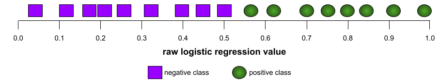
A number between 0.0 and 1.0 representing a binary classification model's ability to separate positive classes from negative classes. The closer the AUC is to 1.0, the better the model's ability to separate classes from each other.
For example, the following illustration shows a classification model that separates positive classes (green ovals) from negative classes (purple rectangles) perfectly. This unrealistically perfect model has an AUC of 1.0:
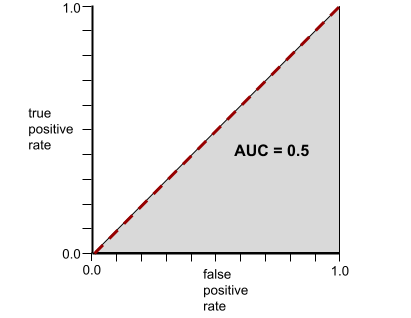
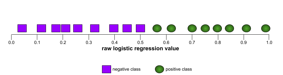
Conversely, the following illustration shows the results for a classification model that generated random results. This model has an AUC of 0.5:
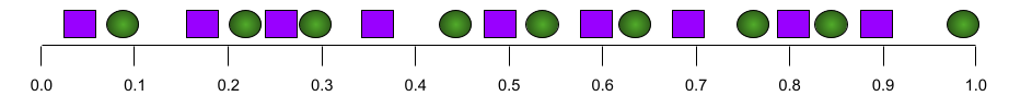
Yes, the preceding model has an AUC of 0.5, not 0.0.
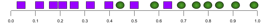
Most models are somewhere between the two extremes. For instance, the following model separates positives from negatives somewhat, and therefore has an AUC somewhere between 0.5 and 1.0:
AUC ignores any value you set for classification threshold. Instead, AUC considers all possible classification thresholds.
Click the icon to learn about the relationship between AUC and ROC curves.
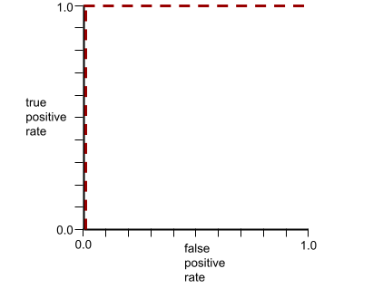
AUC represents the area under an ROC curve. For example, the ROC curve for a model that perfectly separates positives from negatives looks as follows:
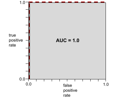
AUC is the area of the gray region in the preceding illustration. In this unusual case, the area is simply the length of the gray region (1.0) multiplied by the width of the gray region (1.0). So, the product of 1.0 and 1.0 yields an AUC of exactly 1.0, which is the highest possible AUC score.
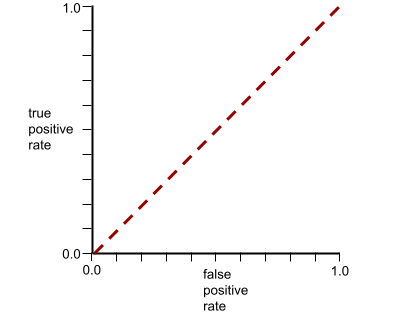
Conversely, the ROC curve for a classification model that can't separate classes at all is as follows. The area of this gray region is 0.5.
A more typical ROC curve looks approximately like the following:
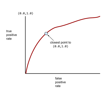
It would be painstaking to calculate the area under this curve manually, which is why a program typically calculates most AUC values.
See Classification: ROC and AUC in Machine Learning Crash Course for more information.
average precision at k
A metric for summarizing a model's performance on a single prompt that generates ranked results, such as a numbered list of book recommendations. Average precision at k is, well, the average of the precision at k values for each relevant result. The formula for average precision at k is therefore:
\[{\text{average precision at k}} = \frac{1}{n} \sum_{i=1}^n {\text{precision at k for each relevant item} } \]
where:
- \(n\) is the number of relevant items in the list.
Contrast with recall at k.
B
baseline
A model used as a reference point for comparing how well another model (typically, a more complex one) is performing. For example, a logistic regression model might serve as a good baseline for a deep model.
For a particular problem, the baseline helps model developers quantify the minimal expected performance that a new model must achieve for the new model to be useful.
Boolean Questions (BoolQ)
A dataset for evaluating an LLM's proficiency in answering yes-or-no questions. Each of the challenges in the dataset has three components:
- A query
- A passage implying the answer to the query.
- The correct answer, which is either yes or no.
For example:
- Query: Are there any nuclear power plants in Michigan?
- Passage: ...three nuclear power plants supply Michigan with about 30% of its electricity.
- Correct answer: Yes
Researchers gathered the questions from anonymized, aggregated Google Search queries and then used Wikipedia pages to ground the information.
For more information, see BoolQ: Exploring the Surprising Difficulty of Natural Yes/No Questions.
BoolQ is a component of the SuperGLUE ensemble.
BoolQ
Abbreviation for Boolean Questions.
C
CB
Abbreviation for CommitmentBank.
Character N-gram F-score (ChrF)
A metric to evaluate machine translation models. Character N-gram F-score determines the degree to which N-grams in reference text overlap the N-grams in an ML model's generated text.
Character N-gram F-score is similar to metrics in the ROUGE and BLEU families, except that:
- Character N-gram F-score operates on character N-grams.
- ROUGE and BLEU operate on word N-grams or tokens.
Choice of Plausible Alternatives (COPA)
A dataset for evaluating how well an LLM can identify the better of two alternative answers to a premise. Each of the challenges in the dataset consists of three components:
- A premise, which is typically a statement followed by a question
- Two possible answers to the question posed in the premise, one of which is correct and the other incorrect
- The correct answer
For example:
- Premise: The man broke his toe. What was the CAUSE of this?
- Possible answers:
- He got a hole in his sock.
- He dropped a hammer on his foot.
- Correct answer: 2
COPA is a component of the SuperGLUE ensemble.
CommitmentBank (CB)
A dataset for evaluating an LLM's proficiency in determining whether the author of a passage believes a target clause within that passage. Each entry in the dataset contains:
- A passage
- A target clause within that passage
- A Boolean value indicating whether the passage's author believes the target clause
For example:
- Passage: What fun to hear Artemis laugh. She's such a serious child. I didn't know she had a sense of humor.
- Target clause: she had a sense of humor
- Boolean: True, which means the author believes the target clause
CommitmentBank is a component of the SuperGLUE ensemble.
COPA
Abbreviation for Choice of Plausible Alternatives.
cost
Synonym for loss.
counterfactual fairness
A fairness metric that checks whether a classification model produces the same result for one individual as it does for another individual who is identical to the first, except with respect to one or more sensitive attributes. Evaluating a classification model for counterfactual fairness is one method for surfacing potential sources of bias in a model.
See either of the following for more information:
- Fairness: Counterfactual fairness in Machine Learning Crash Course.
- When Worlds Collide: Integrating Different Counterfactual Assumptions in Fairness
cross-entropy
A generalization of Log Loss to multi-class classification problems. Cross-entropy quantifies the difference between two probability distributions. See also perplexity.
cumulative distribution function (CDF)
A function that defines the frequency of samples less than or equal to a target value. For example, consider a normal distribution of continuous values. A CDF tells you that approximately 50% of samples should be less than or equal to the mean and that approximately 84% of samples should be less than or equal to one standard deviation above the mean.
D
demographic parity
A fairness metric that is satisfied if the results of a model's classification are not dependent on a given sensitive attribute.
For example, if both Lilliputians and Brobdingnagians apply to Glubbdubdrib University, demographic parity is achieved if the percentage of Lilliputians admitted is the same as the percentage of Brobdingnagians admitted, irrespective of whether one group is on average more qualified than the other.
Contrast with equalized odds and equality of opportunity, which permit classification results in aggregate to depend on sensitive attributes, but don't permit classification results for certain specified ground truth labels to depend on sensitive attributes. See "Attacking discrimination with smarter machine learning" for a visualization exploring the tradeoffs when optimizing for demographic parity.
See Fairness: demographic parity in Machine Learning Crash Course for more information.
E
earth mover's distance (EMD)
A measure of the relative similarity of two distributions. The lower the earth mover's distance, the more similar the distributions.
edit distance
A measurement of how similar two text strings are to each other. In machine learning, edit distance is useful for the following reasons:
- Edit distance is easy to compute.
- Edit distance can compare two strings known to be similar to each other.
- Edit distance can determine the degree to which different strings are similar to a given string.
Several definitions of edit distance exist, each using different string operations. See Levenshtein distance for an example.
empirical cumulative distribution function (eCDF or EDF)
A cumulative distribution function based on empirical measurements from a real dataset. The value of the function at any point along the x-axis is the fraction of observations in the dataset that are less than or equal to the specified value.
entropy
In information theory, a description of how unpredictable a probability distribution is. Alternatively, entropy is also defined as how much information each example contains. A distribution has the highest possible entropy when all values of a random variable are equally likely.
The entropy of a set with two possible values "0" and "1" (for example, the labels in a binary classification problem) has the following formula:
H = -p log p - q log q = -p log p - (1-p) * log (1-p)
where:
- H is the entropy.
- p is the fraction of "1" examples.
- q is the fraction of "0" examples. Note that q = (1 - p)
- log is generally log2. In this case, the entropy unit is a bit.
For example, suppose the following:
- 100 examples contain the value "1"
- 300 examples contain the value "0"
Therefore, the entropy value is:
- p = 0.25
- q = 0.75
- H = (-0.25)log2(0.25) - (0.75)log2(0.75) = 0.81 bits per example
A set that is perfectly balanced (for example, 200 "0"s and 200 "1"s) would have an entropy of 1.0 bit per example. As a set becomes more imbalanced, its entropy moves towards 0.0.
In decision trees, entropy helps formulate information gain to help the splitter select the conditions during the growth of a classification decision tree.
Compare entropy with:
- gini impurity
- cross-entropy loss function
Entropy is often called Shannon's entropy.
See Exact splitter for binary classification with numerical features in the Decision Forests course for more information.
equality of opportunity
A fairness metric to assess whether a model is predicting the desirable outcome equally well for all values of a sensitive attribute. In other words, if the desirable outcome for a model is the positive class, the goal would be to have the true positive rate be the same for all groups.
Equality of opportunity is related to equalized odds, which requires that both the true positive rates and false positive rates are the same for all groups.
Suppose Glubbdubdrib University admits both Lilliputians and Brobdingnagians to a rigorous mathematics program. Lilliputians' secondary schools offer a robust curriculum of math classes, and the vast majority of students are qualified for the university program. Brobdingnagians' secondary schools don't offer math classes at all, and as a result, far fewer of their students are qualified. Equality of opportunity is satisfied for the preferred label of "admitted" with respect to nationality (Lilliputian or Brobdingnagian) if qualified students are equally likely to be admitted irrespective of whether they're a Lilliputian or a Brobdingnagian.
For example, suppose 100 Lilliputians and 100 Brobdingnagians apply to Glubbdubdrib University, and admissions decisions are made as follows:
Table 1. Lilliputian applicants (90% are qualified)
| Qualified | Unqualified | |
|---|---|---|
| Admitted | 45 | 3 |
| Rejected | 45 | 7 |
| Total | 90 | 10 |
|
Percentage of qualified students admitted: 45/90 = 50% Percentage of unqualified students rejected: 7/10 = 70% Total percentage of Lilliputian students admitted: (45+3)/100 = 48% |
||
Table 2. Brobdingnagian applicants (10% are qualified):
| Qualified | Unqualified | |
|---|---|---|
| Admitted | 5 | 9 |
| Rejected | 5 | 81 |
| Total | 10 | 90 |
|
Percentage of qualified students admitted: 5/10 = 50% Percentage of unqualified students rejected: 81/90 = 90% Total percentage of Brobdingnagian students admitted: (5+9)/100 = 14% |
||
The preceding examples satisfy equality of opportunity for acceptance of qualified students because qualified Lilliputians and Brobdingnagians both have a 50% chance of being admitted.
While equality of opportunity is satisfied, the following two fairness metrics are not satisfied:
- demographic parity: Lilliputians and Brobdingnagians are admitted to the university at different rates; 48% of Lilliputians students are admitted, but only 14% of Brobdingnagian students are admitted.
- equalized odds: While qualified Lilliputian and Brobdingnagian students both have the same chance of being admitted, the additional constraint that unqualified Lilliputians and Brobdingnagians both have the same chance of being rejected is not satisfied. Unqualified Lilliputians have a 70% rejection rate, whereas unqualified Brobdingnagians have a 90% rejection rate.
See Fairness: Equality of opportunity in Machine Learning Crash Course for more information.
equalized odds
A fairness metric to assess whether a model is predicting outcomes equally well for all values of a sensitive attribute with respect to both the positive class and negative class—not just one class or the other exclusively. In other words, both the true positive rate and false negative rate should be the same for all groups.
Equalized odds is related to equality of opportunity, which only focuses on error rates for a single class (positive or negative).
For example, suppose Glubbdubdrib University admits both Lilliputians and Brobdingnagians to a rigorous mathematics program. Lilliputians' secondary schools offer a robust curriculum of math classes, and the vast majority of students are qualified for the university program. Brobdingnagians' secondary schools don't offer math classes at all, and as a result, far fewer of their students are qualified. Equalized odds is satisfied provided that no matter whether an applicant is a Lilliputian or a Brobdingnagian, if they are qualified, they are equally as likely to get admitted to the program, and if they are not qualified, they are equally as likely to get rejected.
Suppose 100 Lilliputians and 100 Brobdingnagians apply to Glubbdubdrib University, and admissions decisions are made as follows:
Table 3. Lilliputian applicants (90% are qualified)
| Qualified | Unqualified | |
|---|---|---|
| Admitted | 45 | 2 |
| Rejected | 45 | 8 |
| Total | 90 | 10 |
|
Percentage of qualified students admitted: 45/90 = 50% Percentage of unqualified students rejected: 8/10 = 80% Total percentage of Lilliputian students admitted: (45+2)/100 = 47% |
||
Table 4. Brobdingnagian applicants (10% are qualified):
| Qualified | Unqualified | |
|---|---|---|
| Admitted | 5 | 18 |
| Rejected | 5 | 72 |
| Total | 10 | 90 |
|
Percentage of qualified students admitted: 5/10 = 50% Percentage of unqualified students rejected: 72/90 = 80% Total percentage of Brobdingnagian students admitted: (5+18)/100 = 23% |
||
Equalized odds is satisfied because qualified Lilliputian and Brobdingnagian students both have a 50% chance of being admitted, and unqualified Lilliputian and Brobdingnagian have an 80% chance of being rejected.
Equalized odds is formally defined in "Equality of Opportunity in Supervised Learning" as follows: "predictor Ŷ satisfies equalized odds with respect to protected attribute A and outcome Y if Ŷ and A are independent, conditional on Y."
evals
Primarily used as an abbreviation for LLM evaluations. More broadly, evals is an abbreviation for any form of evaluation.
evaluation
The process of measuring a model's quality or comparing different models against each other.
To evaluate a supervised machine learning model, you typically judge it against a validation set and a test set. Evaluating a LLM typically involves broader quality and safety assessments.
exact match
An all-or-nothing metric in which the model's output either matches ground truth or the reference text exactly or it doesn't. For example, if ground truth is orange, the only model output that satisfies exact match is orange.
Exact match can also evaluate models whose output is a sequence (a ranked list of items). In general, exact match requires the generated ranked list to exactly match ground truth; that is, each item in both lists must be in the same order. That said, if ground truth consists of multiple correct sequences, then exact match only requires model's output matches one of the correct sequences.
Extreme Summarization (xsum)
A dataset for evaluating an LLM's ability to summarize a single document. Each entry in the dataset consists of:
- A document authored by the British Broadcasting Corporation (BBC).
- A one-sentence summary of that document.
For details, see Don't Give Me the Details, Just the Summary! Topic-Aware Convolutional Neural Networks for Extreme Summarization.
F
F1
A "roll-up" binary classification metric that relies on both precision and recall. Here is the formula:
fairness metric
A mathematical definition of "fairness" that is measurable. Some commonly used fairness metrics include:
Many fairness metrics are mutually exclusive; see incompatibility of fairness metrics.
false negative (FN)
An example in which the model mistakenly predicts the negative class. For example, the model predicts that a particular email message is not spam (the negative class), but that email message actually is spam.
false negative rate
The proportion of actual positive examples for which the model mistakenly predicted the negative class. The following formula calculates the false negative rate:
See Thresholds and the confusion matrix in Machine Learning Crash Course for more information.
false positive (FP)
An example in which the model mistakenly predicts the positive class. For example, the model predicts that a particular email message is spam (the positive class), but that email message is actually not spam.
See Thresholds and the confusion matrix in Machine Learning Crash Course for more information.
false positive rate (FPR)
The proportion of actual negative examples for which the model mistakenly predicted the positive class. The following formula calculates the false positive rate:
The false positive rate is the x-axis in an ROC curve.
See Classification: ROC and AUC in Machine Learning Crash Course for more information.
feature importances
Synonym for variable importances.
foundation model
A very large pre-trained model trained on an enormous and diverse training set. A foundation model can do both of the following:
- Respond well to a wide range of requests.
- Serve as a base model for additional fine-tuning or other customization.
In other words, a foundation model is already very capable in a general sense but can be further customized to become even more useful for a specific task.
fraction of successes
A metric for evaluating an ML model's generated text. The fraction of successes is the number of "successful" generated text outputs divided by the total number of generated text outputs. For example, if a large language model generated 10 blocks of code, five of which were successful, then the fraction of successes would be 50%.
Although fraction of successes is broadly useful throughout statistics, within ML, this metric is primarily useful for measuring verifiable tasks like code generation or math problems.
G
gini impurity
A metric similar to entropy. Splitters use values derived from either gini impurity or entropy to compose conditions for classification decision trees. Information gain is derived from entropy. No universally accepted equivalent term for the metric derived from gini impurity exists; however, this unnamed metric is just as important as information gain.
Gini impurity is also called gini index, or simply gini.
H
hinge loss
A family of loss functions for classification designed to find the decision boundary as distant as possible from each training example, thus maximizing the margin between examples and the boundary. KSVMs use hinge loss (or a related function, such as squared hinge loss). For binary classification, the hinge loss function is defined as follows:
where y is the true label, either -1 or +1, and y' is the raw output of the classification model:
Consequently, a plot of hinge loss versus (y * y') looks as follows:

I
incompatibility of fairness metrics
The idea that some notions of fairness are mutually incompatible and cannot be satisfied simultaneously. As a result, there is no single universal metric for quantifying fairness that can be applied to all ML problems.
While this may seem discouraging, incompatibility of fairness metrics doesn't imply that fairness efforts are fruitless. Instead, it suggests that fairness must be defined contextually for a given ML problem, with the goal of preventing harms specific to its use cases.
See "On the (im)possibility of fairness" for a more detailed discussion of the incompatibility of fairness metrics.
individual fairness
A fairness metric that checks whether similar individuals are classified similarly. For example, Brobdingnagian Academy might want to satisfy individual fairness by ensuring that two students with identical grades and standardized test scores are equally likely to gain admission.
Note that individual fairness relies entirely on how you define "similarity" (in this case, grades and test scores), and you can run the risk of introducing new fairness problems if your similarity metric misses important information (such as the rigor of a student's curriculum).
See "Fairness Through Awareness" for a more detailed discussion of individual fairness.
information gain
In decision forests, the difference between a node's entropy and the weighted (by number of examples) sum of the entropy of its children nodes. A node's entropy is the entropy of the examples in that node.
For example, consider the following entropy values:
- entropy of parent node = 0.6
- entropy of one child node with 16 relevant examples = 0.2
- entropy of another child node with 24 relevant examples = 0.1
So 40% of the examples are in one child node and 60% are in the other child node. Therefore:
- weighted entropy sum of child nodes = (0.4 * 0.2) + (0.6 * 0.1) = 0.14
So, the information gain is:
- information gain = entropy of parent node - weighted entropy sum of child nodes
- information gain = 0.6 - 0.14 = 0.46
Most splitters seek to create conditions that maximize information gain.
inter-rater agreement
A measurement of how often human raters agree when doing a task. If raters disagree, the task instructions may need to be improved. Also sometimes called inter-annotator agreement or inter-rater reliability. See also Cohen's kappa, which is one of the most popular inter-rater agreement measurements.
See Categorical data: Common issues in Machine Learning Crash Course for more information.
L
L1 loss
A loss function that calculates the absolute value of the difference between actual label values and the values that a model predicts. For example, here's the calculation of L1 loss for a batch of five examples:
| Actual value of example | Model's predicted value | Absolute value of delta |
|---|---|---|
| 7 | 6 | 1 |
| 5 | 4 | 1 |
| 8 | 11 | 3 |
| 4 | 6 | 2 |
| 9 | 8 | 1 |
| 8 = L1 loss | ||
L1 loss is less sensitive to outliers than L2 loss.
The Mean Absolute Error is the average L1 loss per example.
See Linear regression: Loss in Machine Learning Crash Course for more information.
L2 loss
A loss function that calculates the square of the difference between actual label values and the values that a model predicts. For example, here's the calculation of L2 loss for a batch of five examples:
| Actual value of example | Model's predicted value | Square of delta |
|---|---|---|
| 7 | 6 | 1 |
| 5 | 4 | 1 |
| 8 | 11 | 9 |
| 4 | 6 | 4 |
| 9 | 8 | 1 |
| 16 = L2 loss | ||
Due to squaring, L2 loss amplifies the influence of outliers. That is, L2 loss reacts more strongly to bad predictions than L1 loss. For example, the L1 loss for the preceding batch would be 8 rather than 16. Notice that a single outlier accounts for 9 of the 16.
Regression models typically use L2 loss as the loss function.
The Mean Squared Error is the average L2 loss per example. Squared loss is another name for L2 loss.
See Logistic regression: Loss and regularization in Machine Learning Crash Course for more information.
LLM evaluations (evals)
A set of metrics and benchmarks for assessing the performance of large language models (LLMs). At a high level, LLM evaluations:
- Help researchers identify areas where LLMs need improvement.
- Are useful in comparing different LLMs and identifying the best LLM for a particular task.
- Help ensure that LLMs are safe and ethical to use.
See Large language models (LLMs) in Machine Learning Crash Course for more information.
loss
During the training of a supervised model, a measure of how far a model's prediction is from its label.
A loss function calculates the loss.
See Linear regression: Loss in Machine Learning Crash Course for more information.
loss function
During training or testing, a mathematical function that calculates the loss on a batch of examples. A loss function returns a lower loss for models that makes good predictions than for models that make bad predictions.
The goal of training is typically to minimize the loss that a loss function returns.
Many different kinds of loss functions exist. Pick the appropriate loss function for the kind of model you are building. For example:
- L2 loss (or Mean Squared Error) is the loss function for linear regression.
- Log Loss is the loss function for logistic regression.
M
MBPP
Abbreviation for Mostly Basic Python Problems.
Mean Absolute Error (MAE)
The average loss per example when L1 loss is used. Calculate Mean Absolute Error as follows:
- Calculate the L1 loss for a batch.
- Divide the L1 loss by the number of examples in the batch.
For example, consider the calculation of L1 loss on the following batch of five examples:
| Actual value of example | Model's predicted value | Loss (difference between actual and predicted) |
|---|---|---|
| 7 | 6 | 1 |
| 5 | 4 | 1 |
| 8 | 11 | 3 |
| 4 | 6 | 2 |
| 9 | 8 | 1 |
| 8 = L1 loss | ||
So, L1 loss is 8 and the number of examples is 5. Therefore, the Mean Absolute Error is:
Mean Absolute Error = L1 loss / Number of Examples
Mean Absolute Error = 8/5 = 1.6
Contrast Mean Absolute Error with Mean Squared Error and Root Mean Squared Error.
mean average precision at k (mAP@k)
The statistical mean of all average precision at k scores across a validation dataset. One use of mean average precision at k is to judge the quality of recommendations generated by a recommendation system.
Although the phrase "mean average" sounds redundant, the name of the metric is appropriate. After all, this metric finds the mean of multiple average precision at k values.
Mean Squared Error (MSE)
The average loss per example when L2 loss is used. Calculate Mean Squared Error as follows:
- Calculate the L2 loss for a batch.
- Divide the L2 loss by the number of examples in the batch.
For example, consider the loss on the following batch of five examples:
| Actual value | Model's prediction | Loss | Squared loss |
|---|---|---|---|
| 7 | 6 | 1 | 1 |
| 5 | 4 | 1 | 1 |
| 8 | 11 | 3 | 9 |
| 4 | 6 | 2 | 4 |
| 9 | 8 | 1 | 1 |
| 16 = L2 loss | |||
Therefore, the Mean Squared Error is:
Mean Squared Error = L2 loss / Number of Examples
Mean Squared Error = 16/5 = 3.2
Mean Squared Error is a popular training optimizer, particularly for linear regression.
Contrast Mean Squared Error with Mean Absolute Error and Root Mean Squared Error.
TensorFlow Playground uses Mean Squared Error to calculate loss values.
metric
A statistic that you care about.
An objective is a metric that a machine learning system tries to optimize.
Metrics API (tf.metrics)
A TensorFlow API for evaluating models. For example, tf.metrics.accuracy
determines how often a model's predictions match labels.
minimax loss
A loss function for generative adversarial networks, based on the cross-entropy between the distribution of generated data and real data.
Minimax loss is used in the first paper to describe generative adversarial networks.
See Loss Functions in the Generative Adversarial Networks course for more information.
model capacity
The complexity of problems that a model can learn. The more complex the problems that a model can learn, the higher the model's capacity. A model's capacity typically increases with the number of model parameters. For a formal definition of classification model capacity, see VC dimension.
Mostly Basic Python Problems (MBPP)
A dataset for evaluating an LLM's proficiency in generating Python code. Mostly Basic Python Problems provides about 1,000 crowd-sourced programming problems. Each problem in the dataset contains:
- A task description
- Solution code
- Three automated test cases
N
negative class
In binary classification, one class is termed positive and the other is termed negative. The positive class is the thing or event that the model is testing for and the negative class is the other possibility. For example:
- The negative class in a medical test might be "not tumor."
- The negative class in an email classification model might be "not spam."
Contrast with positive class.
O
objective
A metric that your algorithm is trying to optimize.
objective function
The mathematical formula or metric that a model aims to optimize. For example, the objective function for linear regression is usually Mean Squared Loss. Therefore, when training a linear regression model, training aims to minimize Mean Squared Loss.
In some cases, the goal is to maximize the objective function. For example, if the objective function is accuracy, the goal is to maximize accuracy.
See also loss.
P
pass at k (pass@k)
A metric to determine the quality of code (for example, Python) that a large language model generates. More specifically, pass at k tells you the likelihood that at least one generated block of code out of k generated blocks of code will pass all of its unit tests.
Large language models often struggle to generate good code for complex programming problems. Software engineers adapt to this problem by prompting the large language model to generate multiple (k) solutions for the same problem. Then, software engineers test each of the solutions against unit tests. The calculation of pass at k depends on the outcome of the unit tests:
- If one or more of those solutions pass the unit test, then the LLM Passes that code generation challenge.
- If none of the solutions pass the unit test, then the LLM Fails that code generation challenge.
The formula for pass at k is as follows:
\[\text{pass at k} = \frac{\text{total number of passes}} {\text{total number of challenges}}\]
In general, higher values of k produce higher pass at k scores; however, higher values of k require more large language model and unit testing resources.
performance
Overloaded term with the following meanings:
- The standard meaning within software engineering. Namely: How fast (or efficiently) does this piece of software run?
- The meaning within machine learning. Here, performance answers the following question: How correct is this model? That is, how good are the model's predictions?
permutation variable importances
A type of variable importance that evaluates the increase in the prediction error of a model after permuting the feature's values. Permutation variable importance is a model-independent metric.
perplexity
One measure of how well a model is accomplishing its task. For example, suppose your task is to read the first few letters of a word a user is typing on a phone keyboard, and to offer a list of possible completion words. Perplexity, P, for this task is approximately the number of guesses you need to offer in order for your list to contain the actual word the user is trying to type.
Perplexity is related to cross-entropy as follows:
positive class
The class you are testing for.
For example, the positive class in a cancer model might be "tumor." The positive class in an email classification model might be "spam."
Contrast with negative class.
PR AUC (area under the PR curve)
Area under the interpolated precision-recall curve, obtained by plotting (recall, precision) points for different values of the classification threshold.
precision
A metric for classification models that answers the following question:
When the model predicted the positive class, what percentage of the predictions were correct?
Here is the formula:
where:
- true positive means the model correctly predicted the positive class.
- false positive means the model mistakenly predicted the positive class.
For example, suppose a model made 200 positive predictions. Of these 200 positive predictions:
- 150 were true positives.
- 50 were false positives.
In this case:
Contrast with accuracy and recall.
See Classification: Accuracy, recall, precision and related metrics in Machine Learning Crash Course for more information.
precision at k (precision@k)
A metric for evaluating a ranked (ordered) list of items. Precision at k identifies the fraction of the first k items in that list that are "relevant." That is:
\[\text{precision at k} = \frac{\text{relevant items in first k items of the list}} {\text{k}}\]
The value of k must be less than or equal to the length of the returned list. Note that the length of the returned list is not part of the calculation.
Relevance is often subjective; even expert human evaluators often disagree on which items are relevant.
Compare with:
precision-recall curve
A curve of precision versus recall at different classification thresholds.
prediction bias
A value indicating how far apart the average of predictions is from the average of labels in the dataset.
Not to be confused with the bias term in machine learning models or with bias in ethics and fairness.
predictive parity
A fairness metric that checks whether, for a given classification model, the precision rates are equivalent for subgroups under consideration.
For example, a model that predicts college acceptance would satisfy predictive parity for nationality if its precision rate is the same for Lilliputians and Brobdingnagians.
Predictive parity is sometime also called predictive rate parity.
See "Fairness Definitions Explained" (section 3.2.1) for a more detailed discussion of predictive parity.
predictive rate parity
Another name for predictive parity.
probability density function
A function that identifies the frequency of data samples having exactly a
particular value. When a dataset's values are continuous floating-point
numbers, exact matches rarely occur. However, integrating a probability
density function from value x to value y yields the expected frequency of
data samples between x and y.
For example, consider a normal distribution having a mean of 200 and a standard deviation of 30. To determine the expected frequency of data samples falling within the range 211.4 to 218.7, you can integrate the probability density function for a normal distribution from 211.4 to 218.7.
R
Reading Comprehension with Commonsense Reasoning Dataset (ReCoRD)
A dataset to evaluate an LLM's ability to perform commonsense reasoning. Each example in the dataset contains three components:
- A paragraph or two from a news article
- A query in which one of the entities explicitly or implicitly identified in the passage is masked.
- The answer (the name of the entity that belongs in the mask)
See ReCoRD for an extensive list of examples.
ReCoRD is a component of the SuperGLUE ensemble.
RealToxicityPrompts
A dataset that contains a set of sentence beginnings that might contain toxic content. Use this dataset to evaluate an LLM's ability to generate non-toxic text to complete the sentence. Typically, you use the Perspective API to determine how well the LLM performed at this task.
See RealToxicityPrompts: Evaluating Neural Toxic Degeneration in Language Models for details.
recall
A metric for classification models that answers the following question:
When ground truth was the positive class, what percentage of predictions did the model correctly identify as the positive class?
Here is the formula:
\[\text{Recall} = \frac{\text{true positives}} {\text{true positives} + \text{false negatives}} \]
where:
- true positive means the model correctly predicted the positive class.
- false negative means that the model mistakenly predicted the negative class.
For instance, suppose your model made 200 predictions on examples for which ground truth was the positive class. Of these 200 predictions:
- 180 were true positives.
- 20 were false negatives.
In this case:
\[\text{Recall} = \frac{\text{180}} {\text{180} + \text{20}} = 0.9 \]
See Classification: Accuracy, recall, precision and related metrics for more information.
recall at k (recall@k)
A metric for evaluating systems that output a ranked (ordered) list of items. Recall at k identifies the fraction of relevant items in the first k items in that list out of the total number of relevant items returned.
\[\text{recall at k} = \frac{\text{relevant items in first k items of the list}} {\text{total number of relevant items in the list}}\]
Contrast with precision at k.
Recognizing Textual Entailment (RTE)
A dataset for evaluating an LLM's ability to determine whether a hypothesis can be entailed (logically drawn) from a text passage. Each example in an RTE evaluation consists of three parts:
- A passage, typically from news or Wikipedia articles
- A hypothesis
- The correct answer, which is either:
- True, meaning the hypothesis can be entailed from the passage
- False, meaning the hypothesis can't be entailed from the passage
For example:
- Passage: The Euro is the currency of the European Union.
- Hypothesis: France uses the Euro as currency.
- Entailment: True, because France is part of the European Union.
RTE is a component of the SuperGLUE ensemble.
ReCoRD
Abbreviation for Reading Comprehension with Commonsense Reasoning Dataset.
ROC (receiver operating characteristic) Curve
A graph of true positive rate versus false positive rate for different classification thresholds in binary classification.
The shape of an ROC curve suggests a binary classification model's ability to separate positive classes from negative classes. Suppose, for example, that a binary classification model perfectly separates all the negative classes from all the positive classes:
The ROC curve for the preceding model looks as follows:
In contrast, the following illustration graphs the raw logistic regression values for a terrible model that can't separate negative classes from positive classes at all:
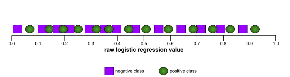
The ROC curve for this model looks as follows:
Meanwhile, back in the real world, most binary classification models separate positive and negative classes to some degree, but usually not perfectly. So, a typical ROC curve falls somewhere between the two extremes:
The point on an ROC curve closest to (0.0,1.0) theoretically identifies the ideal classification threshold. However, several other real-world issues influence the selection of the ideal classification threshold. For example, perhaps false negatives cause far more pain than false positives.
A numerical metric called AUC summarizes the ROC curve into a single floating-point value.
Root Mean Squared Error (RMSE)
The square root of the Mean Squared Error.
ROUGE (Recall-Oriented Understudy for Gisting Evaluation)
A family of metrics that evaluate automatic summarization and machine translation models. ROUGE metrics determine the degree to which a reference text overlaps an ML model's generated text. Each member of the ROUGE family measures overlap in a different way. Higher ROUGE scores indicate more similarity between the reference text and generated text than lower ROUGE scores.
Each ROUGE family member typically generates the following metrics:
- Precision
- Recall
- F1
For details and examples, see:
ROUGE-L
A member of the ROUGE family focused on the length of the longest common subsequence in the reference text and generated text. The following formulas calculate recall and precision for ROUGE-L:
You can then use F1 to roll up ROUGE-L recall and ROUGE-L precision into a single metric:
ROUGE-L ignores any newlines in the reference text and generated text, so the longest common subsequence could cross multiple sentences. When the reference text and generated text involve multiple sentences, a variation of ROUGE-L called ROUGE-Lsum is generally a better metric. ROUGE-Lsum determines the longest common subsequence for each sentence in a passage and then calculates the mean of those longest common subsequences.
ROUGE-N
A set of metrics within the ROUGE family that compares the shared N-grams of a certain size in the reference text and generated text. For example:
- ROUGE-1 measures the number of shared tokens in the reference text and generated text.
- ROUGE-2 measures the number of shared bigrams (2-grams) in the reference text and generated text.
- ROUGE-3 measures the number of shared trigrams (3-grams) in the reference text and generated text.
You can use the following formulas to calculate ROUGE-N recall and ROUGE-N precision for any member of the ROUGE-N family:
You can then use F1 to roll up ROUGE-N recall and ROUGE-N precision into a single metric:
ROUGE-S
A forgiving form of ROUGE-N that enables skip-gram matching. That is, ROUGE-N only counts N-grams that match exactly, but ROUGE-S also counts N-grams separated by one or more words. For example, consider the following:
- reference text: White clouds
- generated text: White billowing clouds
When calculating ROUGE-N, the 2-gram, White clouds doesn't match White billowing clouds. However, when calculating ROUGE-S, White clouds does match White billowing clouds.
R-squared
A regression metric indicating how much variation in a label is due to an individual feature or to a feature set. R-squared is a value between 0 and 1, which you can interpret as follows:
- An R-squared of 0 means that none of a label's variation is due to the feature set.
- An R-squared of 1 means that all of a label's variation is due to the feature set.
- An R-squared between 0 and 1 indicates the extent to which the label's variation can be predicted from a particular feature or the feature set. For example, an R-squared of 0.10 means that 10 percent of the variance in the label is due to the feature set, an R-squared of 0.20 means that 20 percent is due to the feature set, and so on.
R-squared is the square of the Pearson correlation coefficient between the values that a model predicted and ground truth.
RTE
Abbreviation for Recognizing Textual Entailment.
S
scoring
The part of a recommendation system that provides a value or ranking for each item produced by the candidate generation phase.
similarity measure
In clustering algorithms, the metric used to determine how alike (how similar) any two examples are.
sparsity
The number of elements set to zero (or null) in a vector or matrix divided by the total number of entries in that vector or matrix. For example, consider a 100-element matrix in which 98 cells contain zero. The calculation of sparsity is as follows:
Feature sparsity refers to the sparsity of a feature vector; model sparsity refers to the sparsity of the model weights.
SQuAD
Acronym for Stanford Question Answering Dataset, introduced in the paper SQuAD: 100,000+ Questions for Machine Comprehension of Text. The questions in this dataset come from people posing questions about Wikipedia articles. Some of the questions in SQuAD have answers, but other questions intentionally don't have answers. Therefore, you can use SQuAD to evaluate an LLM's ability to do both of the following:
- Answer questions that can be answered.
- Identify questions that cannot be answered.
Exact match in combination with F1 are the most common metrics for evaluating LLMs against SQuAD.
squared hinge loss
The square of the hinge loss. Squared hinge loss penalizes outliers more harshly than regular hinge loss.
squared loss
Synonym for L2 loss.
SuperGLUE
An ensemble of datasets for rating an LLM's overall ability to understand and generate text. The ensemble consists of the following datasets:
- Boolean Questions (BoolQ)
- CommitmentBank (CB)
- Choice of Plausible Alternatives (COPA)
- Multi-sentence Reading Comprehension (MultiRC)
- Reading Comprehension with Commonsense Reasoning Dataset (ReCoRD)
- Recognizing Textual Entailment (RTE)
- Words in Context (WiC)
- Winograd Schema Challenge (WSC)
For details, see SuperGLUE: A Stickier Benchmark for General-Purpose Language Understanding Systems.
T
test loss
A metric representing a model's loss against the test set. When building a model, you typically try to minimize test loss. That's because a low test loss is a stronger quality signal than a low training loss or low validation loss.
A large gap between test loss and training loss or validation loss sometimes suggests that you need to increase the regularization rate.
top-k accuracy
The percentage of times that a "target label" appears within the first k positions of generated lists. The lists could be personalized recommendations or a list of items ordered by softmax.
Top-k accuracy is also known as accuracy at k.
toxicity
The degree to which content is abusive, threatening, or offensive. Many machine learning models can identify, measure, and classify toxicity. Most of these models identify toxicity along multiple parameters, such as the level of abusive language and the level of threatening language.
training loss
A metric representing a model's loss during a particular training iteration. For example, suppose the loss function is Mean Squared Error. Perhaps the training loss (the Mean Squared Error) for the 10th iteration is 2.2, and the training loss for the 100th iteration is 1.9.
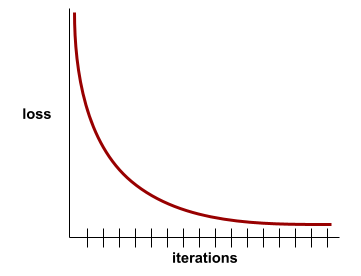
A loss curve plots training loss versus the number of iterations. A loss curve provides the following hints about training:
- A downward slope implies that the model is improving.
- An upward slope implies that the model is getting worse.
- A flat slope implies that the model has reached convergence.
For example, the following somewhat idealized loss curve shows:
- A steep downward slope during the initial iterations, which implies rapid model improvement.
- A gradually flattening (but still downward) slope until close to the end of training, which implies continued model improvement at a somewhat slower pace then during the initial iterations.
- A flat slope towards the end of training, which suggests convergence.
Although training loss is important, see also generalization.
Trivia Question Answering
Datasets to evaluate an LLM's ability to answer trivia questions. Each dataset contains question-answer pairs authored by trivia enthusiasts. Different datasets are grounded by different sources, including:
- Web search (TriviaQA)
- Wikipedia (TriviaQA_wiki)
For more information see TriviaQA: A Large Scale Distantly Supervised Challenge Dataset for Reading Comprehension.
true negative (TN)
An example in which the model correctly predicts the negative class. For example, the model infers that a particular email message is not spam, and that email message really is not spam.
true positive (TP)
An example in which the model correctly predicts the positive class. For example, the model infers that a particular email message is spam, and that email message really is spam.
true positive rate (TPR)
Synonym for recall. That is:
True positive rate is the y-axis in an ROC curve.
Typologically Diverse Question Answering (TyDi QA)
A large dataset for evaluating an LLM's proficiency in answering questions. The dataset contains question and answer pairs in many languages.
For details, see TyDi QA: A Benchmark for Information-Seeking Question Answering in Typologically Diverse Languages.
U
unsupported-claim rate (UCR)
The percentage of claims in a response that aren't grounded. For example, if an LLM's response makes 10 claims but only 1 is grounded, the UCR is 90%.
A high UCR implies that an LLM is hallucinating too frequently.
See also citation precision and citation recall.
V
validation loss
A metric representing a model's loss on the validation set during a particular iteration of training.
See also generalization curve.
variable importances
A set of scores that indicates the relative importance of each feature to the model.
For example, consider a decision tree that estimates house prices. Suppose this decision tree uses three features: size, age, and style. If a set of variable importances for the three features are calculated to be {size=5.8, age=2.5, style=4.7}, then size is more important to the decision tree than age or style.
Different variable importance metrics exist, which can inform ML experts about different aspects of models.
W
Wasserstein loss
One of the loss functions commonly used in generative adversarial networks, based on the earth mover's distance between the distribution of generated data and real data.
WiC
Abbreviation for Words in Context.
WikiLingua (wiki_lingua)
A dataset for evaluating an LLM's ability to summarize short articles. WikiHow, an encyclopedia of articles explaining how to do various tasks, is the human-authored source for both the articles and the summaries. Each entry in the dataset consists of:
- An article, which is created by appending each step of the prose (paragraph) version of the numbered list, minus the opening sentence of each step.
- A summary of that article, consisting of the opening sentence of each step in the numbered list.
For details, see WikiLingua: A New Benchmark Dataset for Cross-Lingual Abstractive Summarization.
Winograd Schema Challenge (WSC)
A format (or dataset conforming to that format) for evaluating an LLM's ability to determine the noun phrase that a pronoun refers to.
Each entry in a Winograd Schema Challenge consists of:
- A short passage, which contains a target pronoun
- A target pronoun
- Candidate noun phrases, followed by the correct answer (a Boolean). If the target pronoun refers to this candidate, the answer is True. If the target pronoun does not refer to this candidate, the answer is False.
For example:
- Passage: Mark told Pete many lies about himself, which Pete included in his book. He should have been more truthful.
- Target pronoun: He
- Candidate noun phrases:
- Mark: True, because the target pronoun refers to Mark
- Pete: False, because the target pronoun doesn't refer to Peter
The Winograd Schema Challenge is a component of the SuperGLUE ensemble.
Words in Context (WiC)
A dataset for evaluating how well an LLM uses context to understand words that have multiple meanings. Each entry in the dataset contains:
- Two sentences, each containing the target word
- The target word
- The correct answer (a Boolean), where:
- True means the target word has the same meaning in the two sentences
- False means the target word has a different meaning in the two sentences
For example:
- Two sentences:
- There's a lot of trash on the bed of the river.
- I keep a glass of water next to my bed when I sleep.
- The target word: bed
- Correct answer: False, because the target word has a different meaning in the two sentences.
For details, see WiC: the Word-in-Context Dataset for Evaluating Context-Sensitive Meaning Representations.
Words in Context is a component of the SuperGLUE ensemble.
WSC
Abbreviation for Winograd Schema Challenge.
X
XL-Sum (xlsum)
A dataset for evaluating an LLM's proficiency in summarizing text. XL-Sum provides entries in many languages. Each entry in the dataset contains:
- An article, taken from the British Broadcasting Company (BBC).
- A summary of the article, written by the article's author. Note that that summary can contain words or phrases not present in the article.
For details, see XL-Sum: Large-Scale Multilingual Abstractive Summarization for 44 Languages.