
借助 Google 表格 API,您可以创建和更新电子表格中的条件格式规则。只有某些格式类型(粗体、斜体、删除线、前景色和背景色)可以通过条件格式进行控制。本页中的示例说明了如何使用 Sheets API 实现常见的条件格式操作。
这些示例以 HTTP 请求的形式呈现,以保持语言中立。如需了解 如何使用 Google API 客户端库以不同语言实现批量更新,请参阅 更新 电子表格。
在这些示例中,占位符 SPREADSHEET_ID 和
SHEET_ID 表示您需要提供这些 ID 的位置。您可以在
电子表格网址中找到
电子表格 ID。您可以使用
spreadsheets.get
方法获取sheet
ID。范围使用 A1
表示法指定。示例范围为 Sheet1!A1:D5。
在行中添加条件颜色渐变
以下
spreadsheets.batchUpdate
方法代码示例展示了如何使用
AddConditionalFormatRuleRequest
为
工作表的第 10 行和第 11 行建立新的渐变条件格式规则。第一条规则规定,该行中的单元格的背景色将根据其值进行设置。该行中的最低值将以深红色着色,而最高值将以亮绿色着色。其他值的颜色将以插值方式呈现。第二条规则执行相同的操作,但使用特定的数值来确定渐变端点(以及不同的颜色)。该请求使用
sheets.InterpolationPointType
作为 type。
请求协议如下所示。
POST https://sheets.googleapis.com/v4/spreadsheets/SPREADSHEET_ID:batchUpdate
{
  "requests": [
    {
      "addConditionalFormatRule": {
        "rule": {
          "ranges": [
            {
              "sheetId": SHEET_ID,
              "startRowIndex": 9,
              "endRowIndex": 10,
            }
          ],
          "gradientRule": {
            "minpoint": {
              "color": {
                "green": 0.2,
                "red": 0.8
              },
              "type": "MIN"
            },
            "maxpoint": {
              "color": {
                "green": 0.9
              },
              "type": "MAX"
            },
          }
        },
        "index": 0
      }
    },
    {
      "addConditionalFormatRule": {
        "rule": {
          "ranges": [
            {
              "sheetId": SHEET_ID,
              "startRowIndex": 10,
              "endRowIndex": 11,
            }
          ],
          "gradientRule": {
            "minpoint": {
              "color": {
                "green": 0.8,
                "red": 0.8
              },
              "type": "NUMBER",
              "value": "0"
            },
            "maxpoint": {
              "color": {
                "blue": 0.9,
                "green": 0.5,
                "red": 0.5
              },
              "type": "NUMBER",
              "value": "256"
            },
          }
        },
        "index": 1
      }
    },
  ]
}
请求后,应用格式规则会更新工作表。由于第 11 行中的渐变的最大点设置为 256,因此任何高于该值的值都具有最大点颜色:

为一组范围添加条件格式规则
以下
spreadsheets.batchUpdate
方法代码示例展示了如何使用
AddConditionalFormatRuleRequest
为工作表的 A 列和 C 列建立新的条件格式规则。
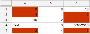
该规则规定,值为 10 或更低的单元格的背景色将更改为深红色。该规则插入在索引 0 处,因此其优先级高于其他格式规则。该请求使用
ConditionType
作为 type 的
BooleanRule。
请求协议如下所示。
POST https://sheets.googleapis.com/v4/spreadsheets/SPREADSHEET_ID:batchUpdate
{
  "requests": [
    {
      "addConditionalFormatRule": {
        "rule": {
          "ranges": [
            {
              "sheetId": SHEET_ID,
              "startColumnIndex": 0,
              "endColumnIndex": 1,
            },
            {
              "sheetId": SHEET_ID,
              "startColumnIndex": 2,
              "endColumnIndex": 3,
            },
          ],
          "booleanRule": {
            "condition": {
              "type": "NUMBER_LESS_THAN_EQ",
              "values": [
                {
                  "userEnteredValue": "10"
                }
              ]
            },
            "format": {
              "backgroundColor": {
                "green": 0.2,
                "red": 0.8,
              }
            }
          }
        },
        "index": 0
      }
    }
  ]
}
请求后,应用格式规则会更新工作表:
为范围添加日期和文本条件格式规则
以下
spreadsheets.batchUpdate
方法代码示例展示了如何使用
AddConditionalFormatRuleRequest
为工作表中的范围 A1:D5 建立新的条件格式规则,
这些规则基于这些单元格中的日期和文本值。如果文本包含字符串“Cost”(不区分大小写),则第一条规则会将单元格文本设置为粗体。如果单元格包含上周之前发生的日期,则第二条规则会将单元格文本设置为斜体并将其着色为蓝色。该请求使用
ConditionType
作为 type 的
BooleanRule。
请求协议如下所示。
POST https://sheets.googleapis.com/v4/spreadsheets/SPREADSHEET_ID:batchUpdate
{
  "requests": [
    {
      "addConditionalFormatRule": {
        "rule": {
          "ranges": [
            {
              "sheetId": SHEET_ID,
              "startRowIndex": 0,
              "endRowIndex": 5,
              "startColumnIndex": 0,
              "endColumnIndex": 4,
            }
          ],
          "booleanRule": {
            "condition": {
              "type": "TEXT_CONTAINS",
              "values": [
                {
                  "userEnteredValue": "Cost"
                }
              ]
            },
            "format": {
              "textFormat": {
                "bold": true
              }
            }
          }
        },
        "index": 0
      }
    },
    {
      "addConditionalFormatRule": {
        "rule": {
          "ranges": [
            {
              "sheetId": SHEET_ID,
              "startRowIndex": 0,
              "endRowIndex": 5,
              "startColumnIndex": 0,
              "endColumnIndex": 4,
            }
          ],
          "booleanRule": {
            "condition": {
              "type": "DATE_BEFORE",
              "values": [
                {
                  "relativeDate": "PAST_WEEK"
                }
              ]
            },
            "format": {
              "textFormat": {
                "italic": true,
                "foregroundColor": {
                  "blue": 1
                }
              }
            }
          }
        },
        "index": 1
      }
    }
  ]
}
请求后,应用格式规则会更新工作表。在此示例中,当前日期为 2016 年 9 月 26 日:

为范围添加自定义公式规则
以下
spreadsheets.batchUpdate
方法代码示例展示了如何使用
AddConditionalFormatRuleRequest
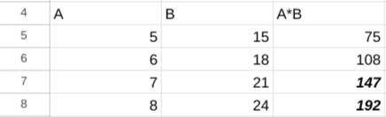
为工作表中的范围 B5:B8 建立新的条件格式规则,
这些规则基于自定义公式。该规则用于计算 A 列和 B 列中单元格的乘积。如果乘积大于 120,则单元格文本将设置为粗体和斜体。该请求使用
ConditionType
作为 type 的
BooleanRule。
请求协议如下所示。
POST https://sheets.googleapis.com/v4/spreadsheets/SPREADSHEET_ID:batchUpdate
{
  "requests": [
    {
      "addConditionalFormatRule": {
        "rule": {
          "ranges": [
            {
              "sheetId": SHEET_ID,
              "startColumnIndex": 2,
              "endColumnIndex": 3,
              "startRowIndex": 4,
              "endRowIndex": 8
            }
          ],
          "booleanRule": {
            "condition": {
              "type": "CUSTOM_FORMULA",
              "values": [
                {
                  "userEnteredValue": "=GT(A5*B5,120)"
                }
              ]
            },
            "format": {
              "textFormat": {
                "bold": true,
                "italic": true
              }
            }
          }
        },
        "index": 0
      }
    }
  ]
}
请求后,应用格式规则会更新工作表:
删除条件格式规则
以下
spreadsheets.batchUpdate
方法代码示例展示了如何使用
DeleteConditionalFormatRuleRequest
删除
由 SHEET_ID 指定的工作表中索引为 0 的条件格式规则。
请求协议如下所示。
POST https://sheets.googleapis.com/v4/spreadsheets/SPREADSHEET_ID:batchUpdate
{
  "requests": [
    {
      "deleteConditionalFormatRule": {
        "sheetId": SHEET_ID,
        "index": 0
      }
    }
  ]
}
读取条件格式规则列表
以下
spreadsheets.get
方法代码示例展示了如何获取电子表格中每个工作表的标题、SHEET_ID和
所有条件格式规则的列表。fields 查询参数用于确定要返回的数据。
请求协议如下所示。
GET https://sheets.googleapis.com/v4/spreadsheets/SPREADSHEET_ID?fields=sheets(properties(title,sheetId),conditionalFormats)
响应由
Spreadsheet资源组成,
该资源包含一个
Sheet对象数组
,每个对象都有一个
SheetProperties
元素和一个
ConditionalFormatRule
元素数组。如果给定的响应字段设置为默认值,则该字段将从响应中省略。该请求使用
ConditionType
作为 type 的
BooleanRule。
{
  "sheets": [
    {
      "properties": {
        "sheetId": 0,
        "title": "Sheet1"
      },
      "conditionalFormats": [
        {
          "ranges": [
            {
              "startRowIndex": 4,
              "endRowIndex": 8,
              "startColumnIndex": 2,
              "endColumnIndex": 3
            }
          ],
          "booleanRule": {
            "condition": {
              "type": "CUSTOM_FORMULA",
              "values": [
                {
                  "userEnteredValue": "=GT(A5*B5,120)"
                }
              ]
            },
            "format": {
              "textFormat": {
                "bold": true,
                "italic": true
              }
            }
          }
        },
        {
          "ranges": [
            {
              "startRowIndex": 0,
              "endRowIndex": 5,
              "startColumnIndex": 0,
              "endColumnIndex": 4
            }
          ],
          "booleanRule": {
            "condition": {
              "type": "DATE_BEFORE",
              "values": [
                {
                  "relativeDate": "PAST_WEEK"
                }
              ]
            },
            "format": {
              "textFormat": {
                "foregroundColor": {
                  "blue": 1
                },
                "italic": true
              }
            }
          }
        },
        ...
      ]
    }
  ]
}
更新条件格式规则或其优先级
以下
spreadsheets.batchUpdate
方法代码示例展示了如何使用
UpdateConditionalFormatRuleRequest
发出多个请求。第一个请求将现有条件格式规则移至更高的索引(从 0 到 2,降低其优先级)。第二个请求将索引 0 处的条件格式规则替换为新规则,该规则用于设置 A1:D5 范围内包含指定的确切文本(“Total Cost”)的单元格的格式。第一个请求的移动操作会在第二个请求开始之前完成,因此第二个请求将替换最初位于索引 1 处的规则。该
请求使用
ConditionType
作为 type 的
BooleanRule。
请求协议如下所示。
POST https://sheets.googleapis.com/v4/spreadsheets/SPREADSHEET_ID:batchUpdate
{
  "requests": [
    {
      "updateConditionalFormatRule": {
        "sheetId": SHEET_ID,
        "index": 0,
        "newIndex": 2
      },
      "updateConditionalFormatRule": {
        "sheetId": SHEET_ID,
        "index": 0,
        "rule": {
          "ranges": [
            {
              "sheetId": SHEET_ID,
              "startRowIndex": 0,
              "endRowIndex": 5,
              "startColumnIndex": 0,
              "endColumnIndex": 4,
            }
          ],
          "booleanRule": {
            "condition": {
              "type": "TEXT_EQ",
              "values": [
                {
                  "userEnteredValue": "Total Cost"
                }
              ]
            },
            "format": {
              "textFormat": {
                "bold": true
              }
            }
          }
        }
      }
    }
  ]
}