一般来说,媒体对 KPI 的影响具有滞后效应,并且会随着时间的推移逐渐减弱。为了对这种滞后效应进行建模,我们通过 Adstock 函数来转换给定渠道的媒体投放情况:
其中:
\(w(s; \alpha) \) 是非负权重函数,
\(x_s \geq 0\) 表示时间 \(s\)时的媒体投放情况,
\(\alpha\ \in\ [0, 1]\) 是衰减形参,
\(L\) 是最大滞后时长。
Meridian 提供两种衰减曲线:几何衰减曲线和二项式衰减曲线。媒体效应的衰减率取决于所选函数以及学习到的形参 alpha。ModelSpec 的 adstock_decay_spec 参数用于定义要使用的函数或函数组合。例如,如需对所有渠道使用二项式衰减,您可以使用:
from meridian.model import spec

model_spec = spec.ModelSpec(
  adstock_decay_spec='binomial'
)
若要对名为 "Channel0"、"Channel1" 和 "Channel2" 的三个渠道分别使用二项式衰减、几何衰减和二项式衰减,您可以指定:
from meridian.model import spec

model_spec = spec.ModelSpec(
  adstock_decay_spec=dict(
    Channel0='binomial',
    Channel1='geometric',
    Channel2='binomial',
  )
)
一般来说,如果您认为媒体渠道的滞后效应中有很大一部分会持续到效应窗口的后半段,建议使用二项式衰减。否则,建议使用几何衰减。
这些函数定义了 Adstock 函数的权重 \(w(s; \alpha)\) 。根据它们的定义,在时间 \(t\),时间 \(t-s\) 的媒体投放具有权重 \(w(s; \alpha) / \sum_{s\in{\{0, ..., L\}}}w(s; \alpha)\)。如需详细了解 Adstock 函数,请参阅媒体饱和与滞后。
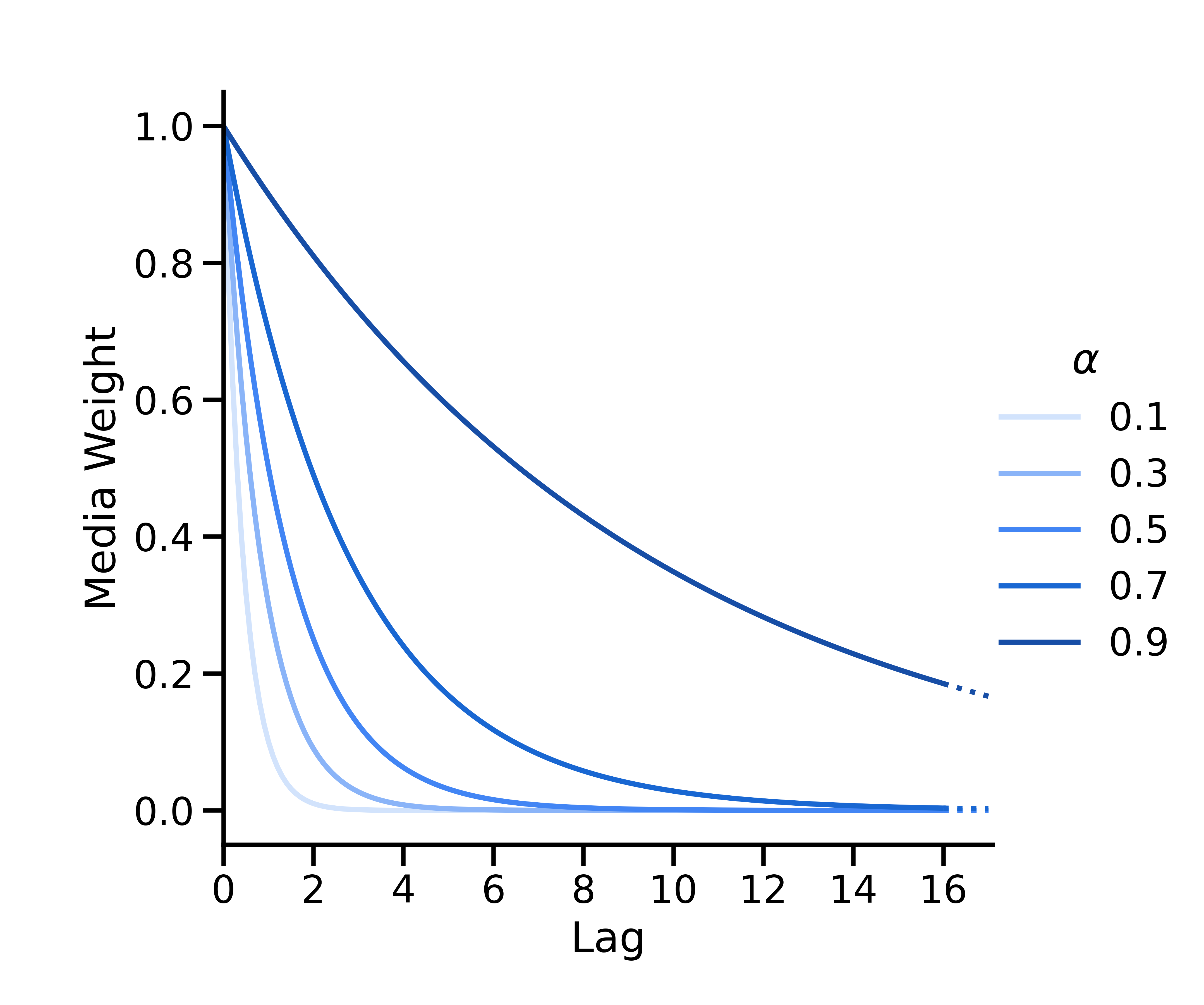
几何衰减
几何衰减的形参为 \(w(s; \alpha) = \alpha^s\),其中\(\alpha \in [0, 1] \) 是表示衰减率的几何形参,\(s\) 是滞后时间。在时间 \(t\),时间 \(t-s\) 的媒体投放具有权重 \(w(s; \alpha) = \alpha^s\),然后再对所有权重进行归一化处理,使它们的总和为 1。
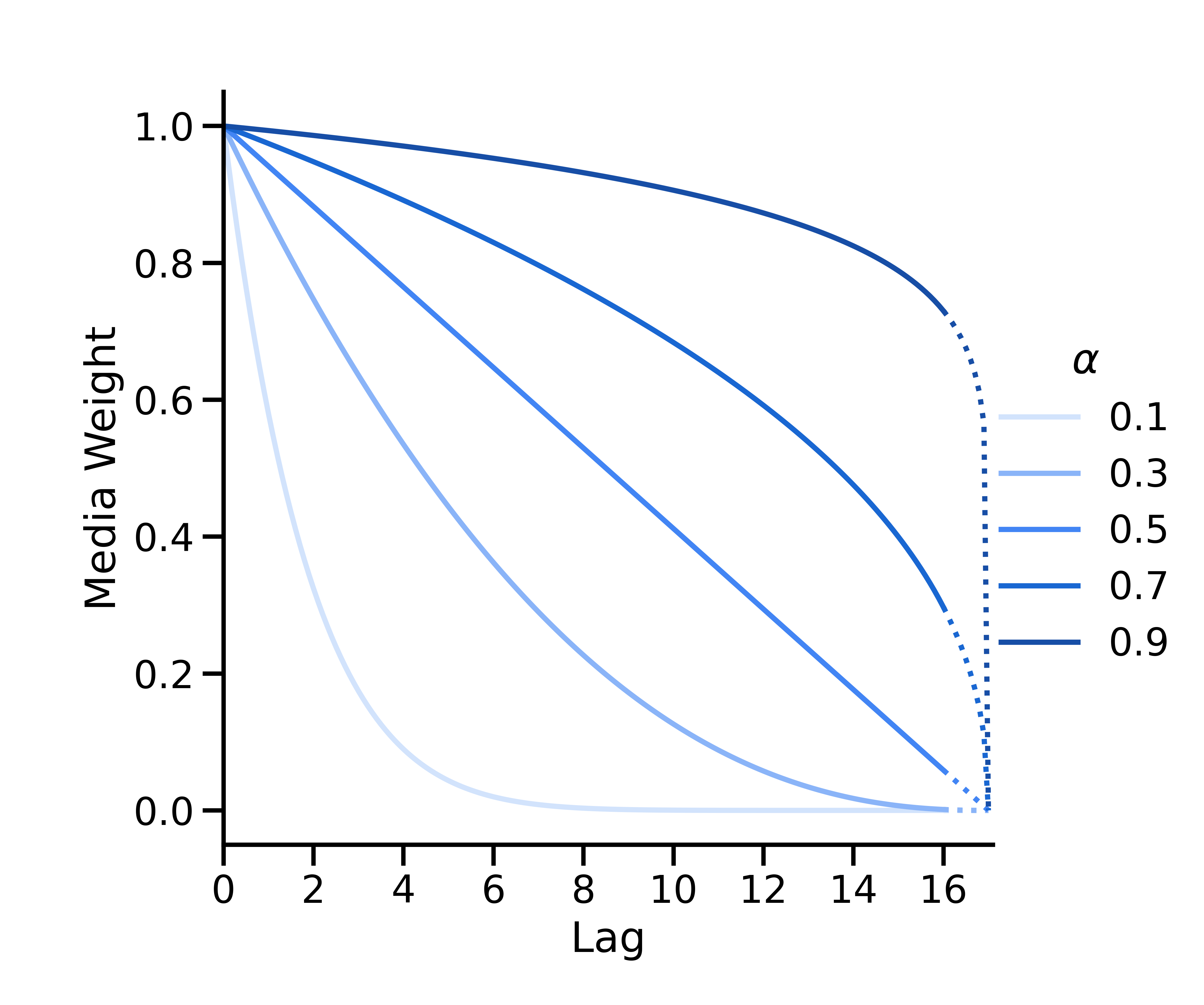
二项式衰减
二项式衰减的形参如下
其中, \(L\) 是最大滞后时间(ModelSpec 的 max_lag 形参)。映射 \(\alpha_*=\frac{1}{\alpha} - 1\) 用于将\(\alpha\) 的值从 \([0, 1]\) 映射到 \([0, \infty)\)。
如果 \(\alpha < 0.5\),二项式曲线为凸曲线;如果 \(\alpha = 0.5\),二项式曲线为线性曲线;如果 \(\alpha > 0.5\),二项式曲线为凹曲线。根据定义,其 x 轴截距始终位于 \(L + 1\)。
在几何衰减和二项式衰减之间做出选择
如果您认为某个渠道很大一部分的效应都在效应窗口的后半段,建议选择二项式衰减。否则,请选择几何衰减。
衰减曲线会影响滞后媒体的相对权重。增加后期时间段的相对权重必然会降低前期时间段的相对权重。二项式衰减曲线定义的权重会比几何曲线更缓慢地衰减到零。因此,二项式衰减曲线会促使渠道总媒体效应的更大一部分发生在后期,而几何衰减曲线会促使渠道总媒体效应的更大一部分发生在前期。如果使用较大的 max_lag 值,二项式衰减曲线是不错的选择,因为它的 x 截距始终位于 \(L + 1\),因此可以“拉伸”以覆盖效应窗口。如需了解更多详情,请参阅设置 max_lag 形参。
由于二项式衰减曲线能够支持较大的 max_lag 值,因此您可能会倾向于为所有渠道选择该曲线。不过,请注意,并非所有渠道都最适合使用二项式衰减曲线进行建模。如果您认为某个渠道有很大一部分效应都在效应窗口的后半段,那么最好使用二项式衰减曲线。错误应用二项式衰减曲线可能会导致低估短期效应。
| 函数 | 几何衰减 | 二项式衰减 |
|---|---|---|
| 最适合的用途 | 具有短期效应的媒体。 | 效应一直持续到效应窗口后半段的媒体。 |
| 曲线形状 | 快速衰减。 | 在衰减之前可以持续更长时间。 |
| 最大滞后时间建议 | 2-10 个时间段。 | 4-20 个时间段。 |
| 缺点 | 容易低估长期效应。 | 容易低估短期效应。 |
关于长期效应的注意事项
若模型中未显现出您所预期的长期效应,可以尝试结合使用二项式衰减曲线、修改 alpha 的先验以及更改 max_lag。借助 MediaEffects.plot_adstock_decay 中的先验曲线,观察 max_lag、alpha 先验和衰减函数之间的相互作用关系。然后,您可以对它们进行微调,使模型符合您对于滞后效应的初始假设。您可以在修改先验和 max_lag 的同时选择特定衰减函数,也可以只修改而不选择衰减函数。建议您尝试不同的组合,以平衡收敛性、模型拟合度和效应窗口。如需详细了解如何选择 max_lag 的值,请参阅设置 max_lag 形参。
Alpha 先验
Meridian 中的默认 alpha 先验为 \(U(0, 1)\),该先验对几何衰减与二项式衰减函数而言均属于无信息先验。如果您对特定渠道的媒体效应衰减率有直观了解,可以为该渠道设置自定义 alpha 先验,以便将您的直观了解告知 Meridian。
对于几何衰减和二项式衰减,\(\alpha\) 与媒体效应衰减率之间存在单调关系: \(\alpha\)越小,衰减越快, \(\alpha\) 越大,衰减越慢。当 \(\alpha=0\)时,几何衰减函数和二项式衰减函数都会最大限度地提高短期效应(此时没有滞后效应);当 \(\alpha=1\)时,它们都会最大限度地提高长期效应(此时历史滞后窗口内的所有媒体都会获得相同的权重)。
因此,我们建议为 alpha 设置一个概率质量更集中于 0 附近的先验分布,以促使效应衰减更快、效应期更短。例如,与默认的均匀分布相比,Beta(1, 3) 分布有更多质量集中于 0 附近。相反,我们建议设置一个概率质量更集中于 1 附近的先验分布,以促使效应衰减更慢、效应期更长。例如,与默认的均匀分布相比,Beta(3, 1) 分布有更多质量集中于 1 附近。我们建议同时绘制 alpha 和媒体权重的先验分布(使用 MediaEffects.plot_adstock_decay),以确认自定义先验分布是否符合您的直觉。
二项式 \(\alpha\) 映射
之所以执行映射 \(\alpha_*: [0, 1]\rightarrow[0, \infty) \) ,是因为二项式函数在 \(\alpha_* \in [0, \infty)\) 范围内衰减,而几何函数在 \(\alpha \in [0, 1]\)范围内衰减。此映射可确保在二项式衰减中,以 \([0, 1]\) 区间定义的先验能正确转换为 \([0, \infty)\) ,并让模型规范与几何衰减保持一致,其中低 alpha 值表示衰减快、效应期短,高 alpha 值表示衰减慢、效应期长。
高级选项:使用二项式衰减时,直接在 \(\alpha_*\) 上设置自定义先验
对于几何函数和二项式函数,Meridian 均在 \(\alpha\) 上使用 \(U(0, 1)\) 的默认先验。对于二项式衰减,\(\alpha\) 上的 \(U(0, 1)\) 先验等效于 \(\alpha_*\)上的 Lomax(1, 1) 先验:
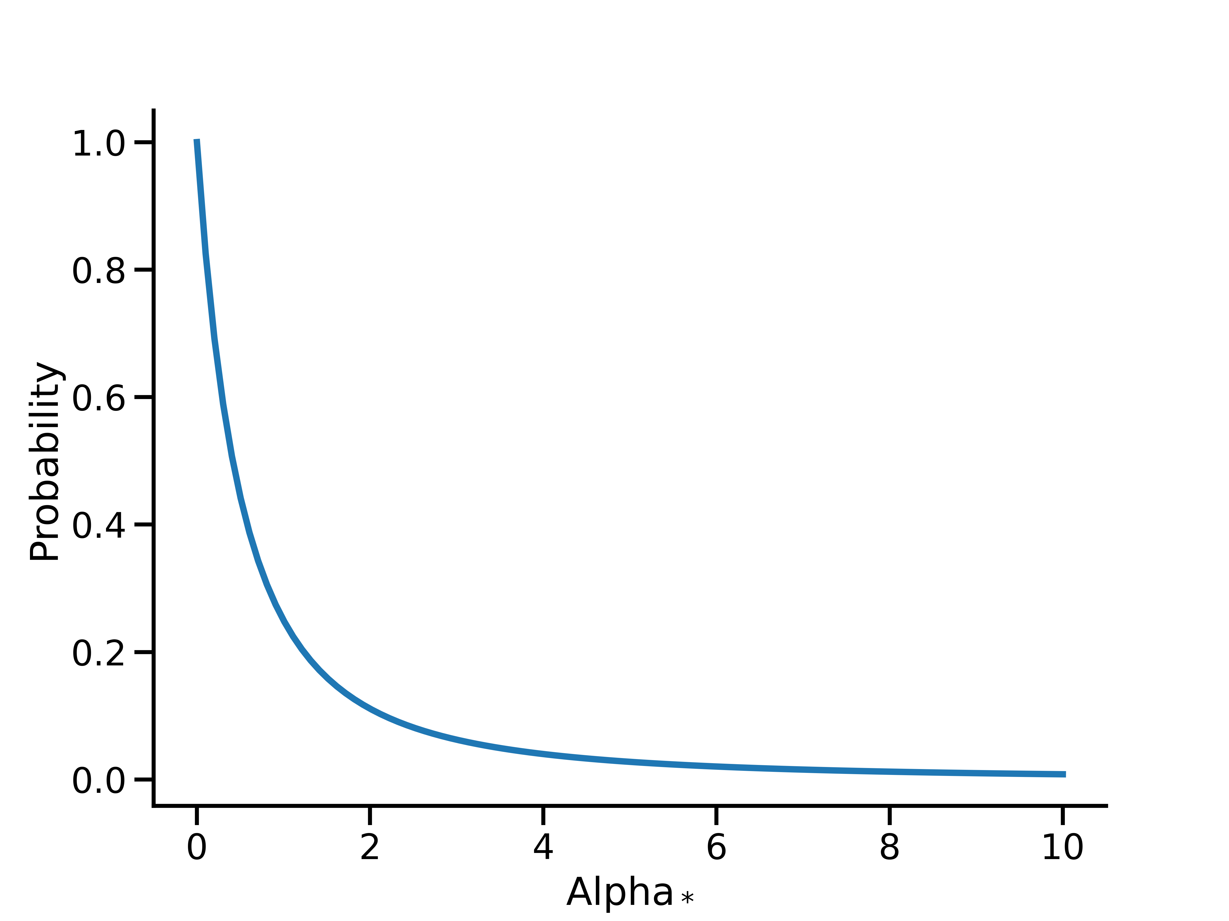
这仍然是一个相对无信息的先验,可让数据通过二项式衰减来确定衰减率。
Meridian 要求自定义 \(\alpha\) 先验支持 \([0, 1]\) (例如,Beta 分布),然后再通过 \(1/x-1\)将其映射到非负实数。不过,如果您希望能够在 \(\alpha_*\) 上定义支持 \([0, \infty)\) 的先验,您可以这样做,然后使用反向映射 \(\frac{1}{1+x}\)对其进行转换。此映射可通过辅助方法 adstock_hill.transform_non_negative_reals_distribution 完成。例如,以下代码可获得平均值为 0.5、方差为 0.5 的 \(\alpha_*\) 对数正态先验:
import tensorflow as tf

# Example: pick mu, sigma so that the mean, variance of alpha_* are both 0.5
mu = -tf.math.log(2.0) - 0.5 * tf.math.log(3.0)
sigma = tf.math.sqrt(tf.math.log(3.0))

alpha_star_prior = tfp.distributions.LogNormal(mu, sigma)  # prior on alpha_* for binomial
alpha_prior = adstock_hill.transform_non_negative_reals_distribution(alpha_star_prior)

prior = prior_distribution.PriorDistribution(
  alpha_m=alpha_prior
)

model_spec = spec.ModelSpec(
  prior=prior,
  adstock_decay_spec='binomial'
)
然后,您还可以直接查询 alpha 先验。例如,以下代码可查看 alpha 的概率密度函数:
import numpy as np
from matplotlib import pyplot as plt

x = np.linspace(0, 1, 100)
fig, ax = plt.subplots(figsize=(8, 6))
ax.plot(x, alpha_prior.prob(x), linewidth=3)
ax.set(xlabel='Alpha', ylabel='Probability')
plt.show()
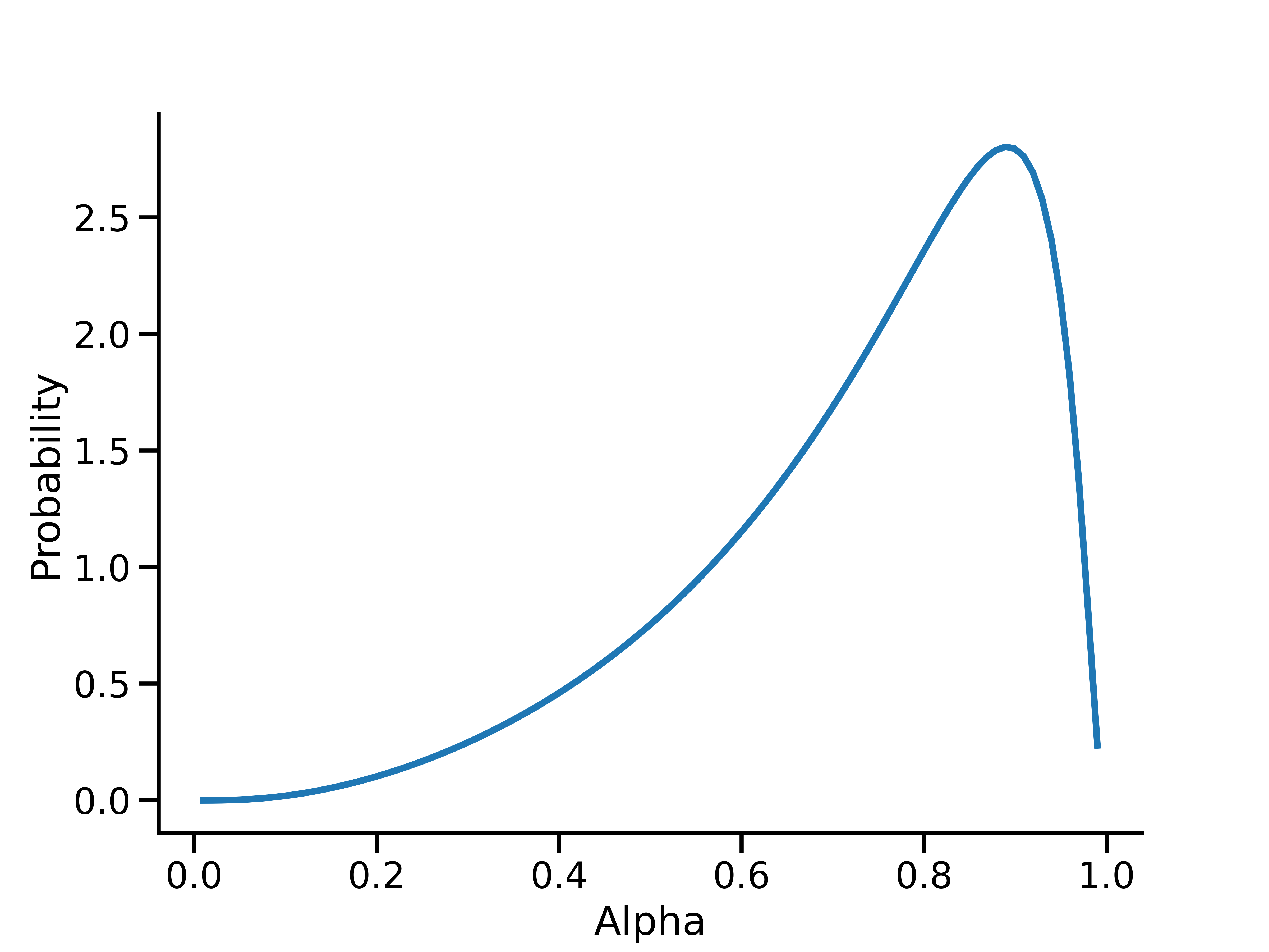
此图显示了 \(\alpha\) 的先验,该先验经转换后可在\(\alpha_*\) 上形成均值为 0.5、方差为 0.5 的对数正态先验。