Implementation of the Thornthwaite-Mather procedure to map groundwater recharge

Groundwater recharge represents the amount of water coming from precipitation reaching the groundwater table. Its determination helps to better understand the available/renewable groundwater in watersheds and the shape of groundwater flow systems.

One of the simplest methods to estimate groundwater recharge is the Thornthwaite-Mather procedure (Steenhuis and Van Der Molen, 1986). This procedure was published by Thornthwaite and Mather (1955, 1957). The idea of this procedure is to calculate the water balance in the root zone of the soil where water can be (1) evaporated into the atmosphere under the effect of heat, (2) transpired by vegetation, (3) stored by the soil, and eventually (4) infiltrated when stored water exceeds the field capacity.

This procedures relies on several parameters and variables described as follows:

• information about soil texture (e.g. sand and clay content) to describe the hydraulic properties of the soil and its capacity to store/infiltrate,
• meteorological records: precipitation and potential evapotranspiration.

Of course groundwater recharge can be influenced by many other factors such as the slope of the terrain, the snow cover, the variability of the crop/land cover and the irrigation. In the following these aspects are not taken into account.

In the first part of the tutorial, the Earth Engine python API will be initialized, some useful libraries will be imported, and the location/period of interest will be defined.

In the second part, OpenLandMap datasets related to soil properties will be explored. The wilting point and field capacity of the soil will be calculated by applying some mathematical expressions to multiple images.

In the third part, evapotranspiration and precipitation datasets will be imported. A function will be defined to resample the time resolution of an ee.ImageCollection and to homogenize time index of both datasets. Both datasets will then be combined into one.

In the fourth and final part, the Thornthwaite-Mather(TM) procedure will be implemented by iterating over the meteorological ee.ImageCollection. Finally, a comparison between groundwater recharge in two places will be described and the resulting mean annual groundwater recharge will be displayed over France.

Run me first

Earth Engine API

First of all, run the following cell to initialize the API. The output will contain instructions on how to grant this notebook access to Earth Engine using your account.

import ee

# Trigger the authentication flow.
ee.Authenticate()

# Initialize the library.
ee.Initialize(project='my-project')

Other libraries

Import other libraries/modules used in this notebook.

• pandas: data analysis (including the DataFrame data structure)
• matplotlib: data visualization library
• numpy: array-processing package
• folium: interactive web map
• pprint: a pretty printer
• branca.colormap: utility module for dealing with colormaps.

import pandas as pd
import matplotlib.pyplot as plt
import numpy as np
import folium
import pprint
import branca.colormap as cm

Some input parameters

We additionally define some parameters used to evaluate the results of our implementation. Particularly:

• the period of interest to get meteorological records,
• a location of interest based on longitude and latitude coordinates. In the following, the point of interest is located in a productive agricultural region which is about 30 kilometers outside of the city of Lyon (France). This point is used to evaluate and illustrate the progress of the described procedure.

# Initial date of interest (inclusive).
i_date = "2015-01-01"

# Final date of interest (exclusive).
f_date = "2020-01-01"

# Define the location of interest with a point.
lon = 5.145041
lat = 45.772439
poi = ee.Geometry.Point(lon, lat)

# A nominal scale in meters of the projection to work in [in meters].
scale = 1000

From soil texture to hydraulic properties

Definitions

Two hydraulic properties of soil are commonly used in the TM procedure:

• the wilting point represents the point below what water cannot be extracted by plant roots,
• the field capacity represents the point after which water cannot be stored by soil any more. After that point, gravitational forces become too high and water starts to infiltrate the lower levels.

Some equations given by Saxton & Rawls (2006) are used to link both parameters to the texture of the soil. The calculation of water content at wilting point \(θ_{WP}\) can be done as follows:

with:

where:

• \(S\): represents the sand content of the soil (mass percentage),
• \(C\): represents the clay content of the soil (mass percentage),
• \(OM\): represents the organic matter content of the soil (mass percentage).

Similarly, the calculation of the water content at field capacity \(θ_{FC}\) can be done as follows:

with:

Determination of soil texture and properties

In the following, OpenLandMap datasets are used to describe clay, sand and organic carbon content of soil. A global dataset of soil water content at the field capacity with a resolution of 250 m has been made available by Hengl & Gupta (2019). However, up to now, there is no dataset dedicated to the water content of soil at the wilting point. Consequently, in the following, both parameters will be determined considering the previous equations and using the global datasets giving the sand, clay and organic matter contents of the soil. According to the description, these datasets are based on machine learning predictions from global compilation of soil profiles and samples. Processing steps are described in detail here. The information (clay, sand content, etc.) is given at 6 standard depths (0, 10, 30, 60, 100 and 200 cm) at 250 m resolution.

These standard depths and associated bands are defined into a list as follows:

# Soil depths [in cm] where we have data.
olm_depths = [0, 10, 30, 60, 100, 200]

# Names of bands associated with reference depths.
olm_bands = ["b" + str(sd) for sd in olm_depths]

We now define a function to get the ee.Image associated to the parameter we are interested in (e.g. sand, clay, organic carbon content, etc.).

def get_soil_prop(param):
    """
    This function returns soil properties image
    param (str): must be one of:
        "sand"     - Sand fraction
        "clay"     - Clay fraction
        "orgc"     - Organic Carbon fraction
    """
    if param == "sand":  # Sand fraction [%w]
        snippet = "OpenLandMap/SOL/SOL_SAND-WFRACTION_USDA-3A1A1A_M/v02"
        # Define the scale factor in accordance with the dataset description.
        scale_factor = 1 * 0.01

    elif param == "clay":  # Clay fraction [%w]
        snippet = "OpenLandMap/SOL/SOL_CLAY-WFRACTION_USDA-3A1A1A_M/v02"
        # Define the scale factor in accordance with the dataset description.
        scale_factor = 1 * 0.01

    elif param == "orgc":  # Organic Carbon fraction [g/kg]
        snippet = "OpenLandMap/SOL/SOL_ORGANIC-CARBON_USDA-6A1C_M/v02"
        # Define the scale factor in accordance with the dataset description.
        scale_factor = 5 * 0.001  # to get kg/kg
    else:
        return print("error")

    # Apply the scale factor to the ee.Image.
    dataset = ee.Image(snippet).multiply(scale_factor)

    return dataset

We apply this function to import soil properties:

# Image associated with the sand content.
sand = get_soil_prop("sand")

# Image associated with the clay content.
clay = get_soil_prop("clay")

# Image associated with the organic carbon content.
orgc = get_soil_prop("orgc")

To illustrate the result, we define a new method for handing Earth Engine tiles and using it to display the clay content of the soil at a given reference depth, to a Leaflet map.

def add_ee_layer(self, ee_image_object, vis_params, name):
    """Adds a method for displaying Earth Engine image tiles to folium map."""
    map_id_dict = ee.Image(ee_image_object).getMapId(vis_params)
    folium.raster_layers.TileLayer(
        tiles=map_id_dict["tile_fetcher"].url_format,
        attr="Map Data &copy; <a href='https://earthengine.google.com/'>Google Earth Engine</a>",
        name=name,
        overlay=True,
        control=True,
    ).add_to(self)


# Add Earth Engine drawing method to folium.
folium.Map.add_ee_layer = add_ee_layer

my_map = folium.Map(location=[lat, lon], zoom_start=3)

# Set visualization parameters.
vis_params = {
    "bands": ["b0"],
    "min": 0.01,
    "max": 1,
    "opacity": 1,
    "palette": ["white", "#464646"],
}

# Add the sand content data to the map object.
my_map.add_ee_layer(sand, vis_params, "Sand Content")

# Add a marker at the location of interest.
folium.Marker([lat, lon], popup="point of interest").add_to(my_map)

# Add a layer control panel to the map.
my_map.add_child(folium.LayerControl())

# Display the map.
display(my_map)

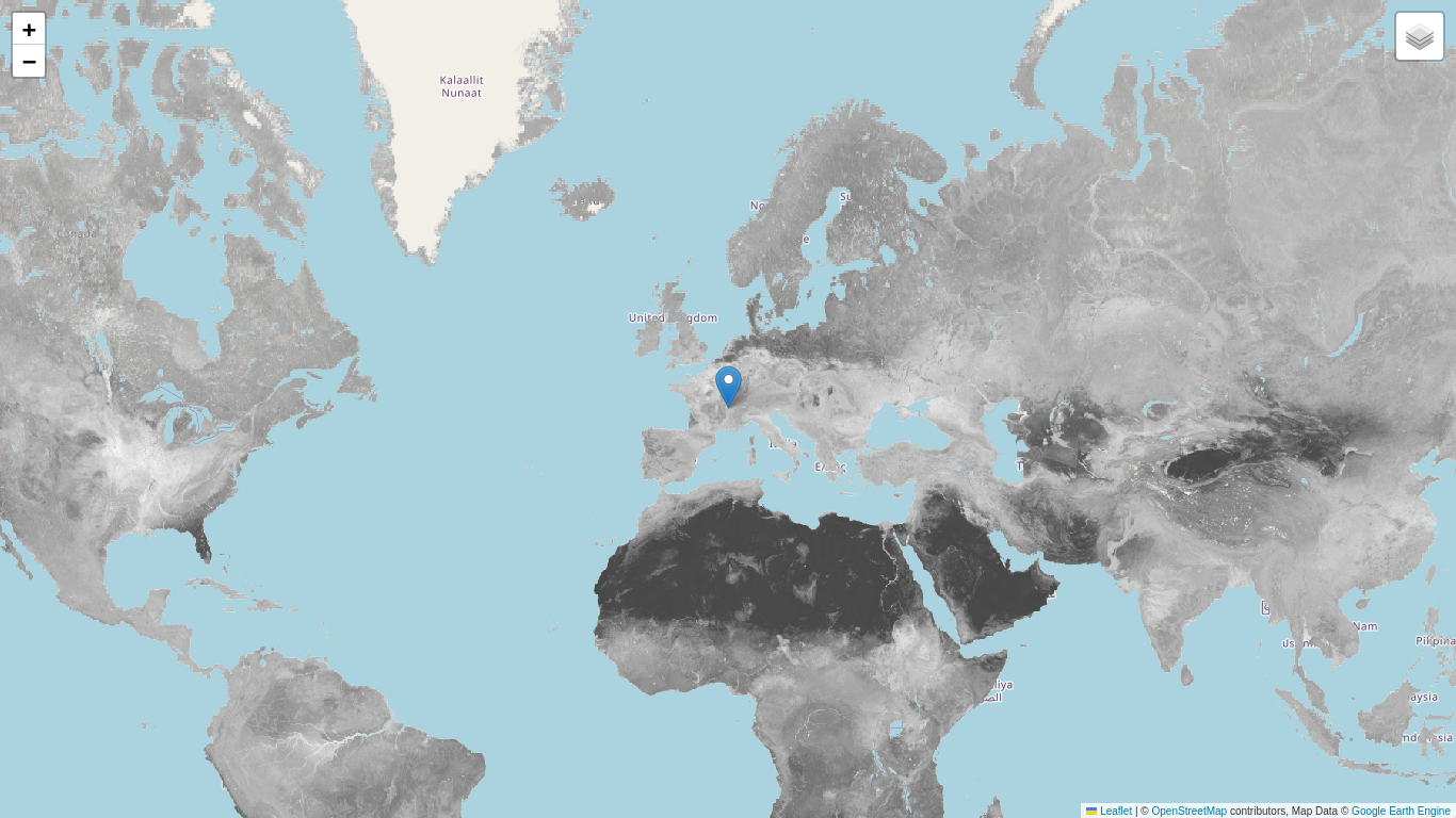
Now, a function is defined to get soil properties at a given location. The following function returns a dictionary indicating the value of the parameter of interest for each standard depth (in centimeter). This function uses the ee.Image.sample method to evaluate the ee.Image properties on the region of interest. The result is then transferred client-side using the ee.Image.getInfo method.

In the example below, we are asking for the sand content.

def local_profile(dataset, poi, buffer):
    # Get properties at the location of interest and transfer to client-side.
    prop = dataset.sample(poi, buffer).select(olm_bands).getInfo()

    # Selection of the features/properties of interest.
    profile = prop["features"][0]["properties"]

    # Re-shaping of the dict.
    profile = {key: round(val, 3) for key, val in profile.items()}

    return profile


# Apply the function to get the sand profile.
profile_sand = local_profile(sand, poi, scale)

# Print the result.
print("Sand content profile at the location of interest:\n", profile_sand)

Sand content profile at the location of interest:
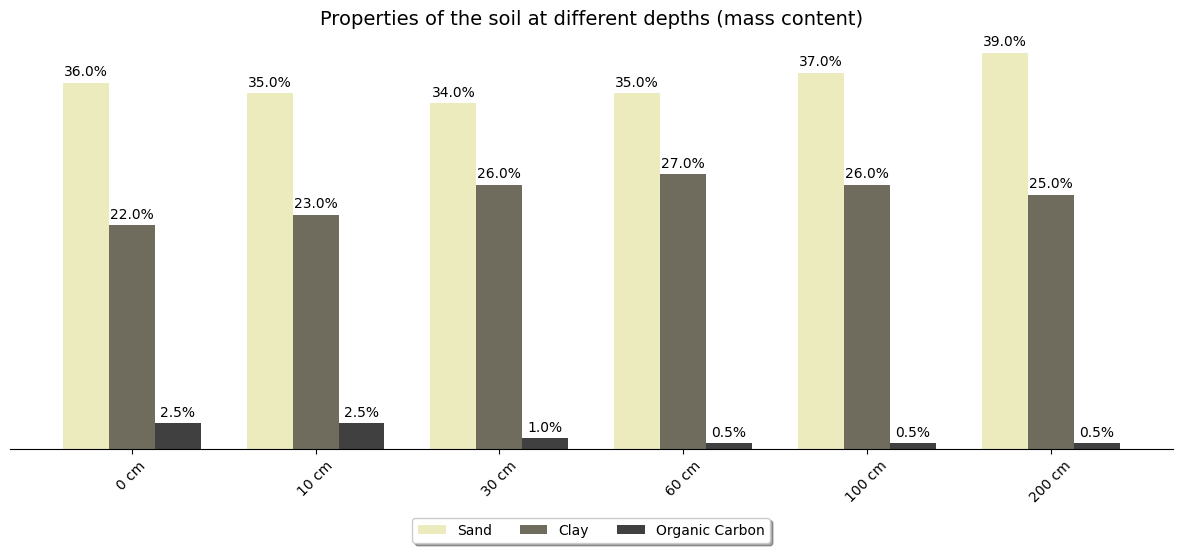
 {'b0': 0.36, 'b10': 0.35, 'b100': 0.37, 'b200': 0.39, 'b30': 0.34, 'b60': 0.35}

We now apply the function to plot the profile of the soil regarding sand and clay and organic carbon content at the location of interest:

# Clay and organic content profiles.
profile_clay = local_profile(clay, poi, scale)
profile_orgc = local_profile(orgc, poi, scale)

# Data visualization in the form of a bar plot.
fig, ax = plt.subplots(figsize=(15, 6))
ax.axes.get_yaxis().set_visible(False)

# Definition of label locations.
x = np.arange(len(olm_bands))

# Definition of the bar width.
width = 0.25

# Bar plot representing the sand content profile.
rect1 = ax.bar(
    x - width,
    [round(100 * profile_sand[b], 2) for b in olm_bands],
    width,
    label="Sand",
    color="#ecebbd",
)

# Bar plot representing the clay content profile.
rect2 = ax.bar(
    x,
    [round(100 * profile_clay[b], 2) for b in olm_bands],
    width,
    label="Clay",
    color="#6f6c5d",
)

# Bar plot representing the organic carbon content profile.
rect3 = ax.bar(
    x + width,
    [round(100 * profile_orgc[b], 2) for b in olm_bands],
    width,
    label="Organic Carbon",
    color="black",
    alpha=0.75,
)

# Definition of a function to attach a label to each bar.
def autolabel_soil_prop(rects):
    """Attach a text label above each bar in *rects*, displaying its height."""
    for rect in rects:
        height = rect.get_height()
        ax.annotate(
            "{}".format(height) + "%",
            xy=(rect.get_x() + rect.get_width() / 2, height),
            xytext=(0, 3),  # 3 points vertical offset.
            textcoords="offset points",
            ha="center",
            va="bottom",
            fontsize=10,
        )


# Application of the function to each barplot.
autolabel_soil_prop(rect1)
autolabel_soil_prop(rect2)
autolabel_soil_prop(rect3)

# Title of the plot.
ax.set_title("Properties of the soil at different depths (mass content)", fontsize=14)

# Properties of x/y labels and ticks.
ax.set_xticks(x)
x_labels = [str(d) + " cm" for d in olm_depths]
ax.set_xticklabels(x_labels, rotation=45, fontsize=10)

ax.spines["left"].set_visible(False)
ax.spines["right"].set_visible(False)
ax.spines["top"].set_visible(False)

# Shrink current axis's height by 10% on the bottom.
box = ax.get_position()
ax.set_position([box.x0, box.y0 + box.height * 0.1, box.width, box.height * 0.9])

# Add a legend below current axis.
ax.legend(
    loc="upper center", bbox_to_anchor=(0.5, -0.15), fancybox=True, shadow=True, ncol=3
)

plt.show()

Expression to calculate hydraulic properties

Now that soil properties are described, the water content at the field capacity and at the wilting point can be calculated according to the equation defined at the beginning of this section. Please note that in the equation of Saxton & Rawls (2006), the wilting point and field capacity are calculated using the Organic Matter content (\(OM\)) and not the Organic Carbon content (\(OC\)). In the following, we convert \(OC\) into \(OM\) using the corrective factor known as the Van Bemmelen factor:

Several operators are available to perform basic mathematical operations on image bands: add(), subtract(), multiply() and divide(). Here, we multiply the organic content by the Van Bemmelen factor. It is done using the ee.Image.multiply method on the organic carbon content ee.Image.

# Conversion of organic carbon content into organic matter content.
orgm = orgc.multiply(1.724)

# Organic matter content profile.
profile_orgm = local_profile(orgm, poi, scale)
print("Organic Matter content profile at the location of interest:\n", profile_orgm)

Organic Matter content profile at the location of interest:
 {'b0': 0.043, 'b10': 0.043, 'b100': 0.009, 'b200': 0.009, 'b30': 0.017, 'b60': 0.009}

When the mathematical operation to apply to the ee.Image becomes too complex, the ee.Image.expression is a good alternative. We use it in the following code block since the calculation of wilting point and field capacity relies on multiple parameters and images. This method takes two arguments:

• a string formalizing the arithmetic expression we want to evaluate,
• a dict associating images to each parameter of the arithmetic expression.

The mathematical expression is applied as follows to determine wilting point and field capacity:

# Initialization of two constant images for wilting point and field capacity.
wilting_point = ee.Image(0)
field_capacity = ee.Image(0)

# Calculation for each standard depth using a loop.
for key in olm_bands:
    # Getting sand, clay and organic matter at the appropriate depth.
    si = sand.select(key)
    ci = clay.select(key)
    oi = orgm.select(key)

    # Calculation of the wilting point.
    # The theta_1500t parameter is needed for the given depth.
    theta_1500ti = (
        ee.Image(0)
        .expression(
            "-0.024 * S + 0.487 * C + 0.006 * OM + 0.005 * (S * OM)\
        - 0.013 * (C * OM) + 0.068 * (S * C) + 0.031",
            {
                "S": si,
                "C": ci,
                "OM": oi,
            },
        )
        .rename("T1500ti")
    )

    # Final expression for the wilting point.
    wpi = theta_1500ti.expression(
        "T1500ti + ( 0.14 * T1500ti - 0.002)", {"T1500ti": theta_1500ti}
    ).rename("wpi")

    # Add as a new band of the global wilting point ee.Image.
    # Do not forget to cast the type with float().
    wilting_point = wilting_point.addBands(wpi.rename(key).float())

    # Same process for the calculation of the field capacity.
    # The parameter theta_33t is needed for the given depth.
    theta_33ti = (
        ee.Image(0)
        .expression(
            "-0.251 * S + 0.195 * C + 0.011 * OM +\
        0.006 * (S * OM) - 0.027 * (C * OM)+\
        0.452 * (S * C) + 0.299",
            {
                "S": si,
                "C": ci,
                "OM": oi,
            },
        )
        .rename("T33ti")
    )

    # Final expression for the field capacity of the soil.
    fci = theta_33ti.expression(
        "T33ti + (1.283 * T33ti * T33ti - 0.374 * T33ti - 0.015)",
        {"T33ti": theta_33ti.select("T33ti")},
    )

    # Add a new band of the global field capacity ee.Image.
    field_capacity = field_capacity.addBands(fci.rename(key).float())

Let's see the result around our location of interest:

profile_wp = local_profile(wilting_point, poi, scale)
profile_fc = local_profile(field_capacity, poi, scale)

print("Wilting point profile:\n", profile_wp)
print("Field capacity profile:\n", profile_fc)

Wilting point profile:
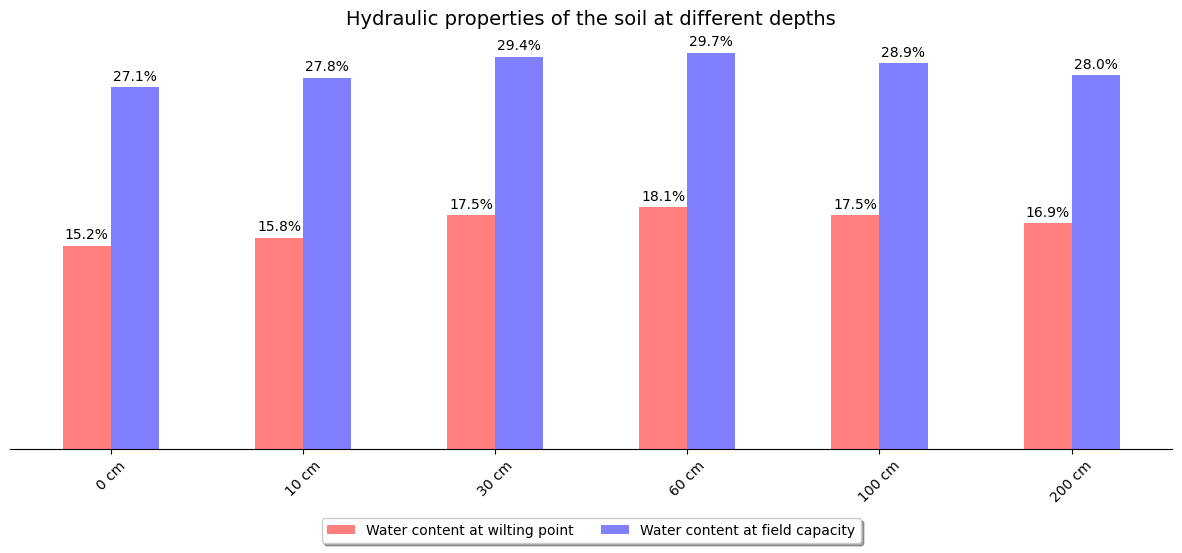
 {'b0': 0.152, 'b10': 0.158, 'b100': 0.175, 'b200': 0.169, 'b30': 0.175, 'b60': 0.181}
Field capacity profile:
 {'b0': 0.271, 'b10': 0.278, 'b100': 0.289, 'b200': 0.28, 'b30': 0.294, 'b60': 0.297}

The result is displayed using barplots as follows:

fig, ax = plt.subplots(figsize=(15, 6))
ax.axes.get_yaxis().set_visible(False)

# Definition of the label locations.
x = np.arange(len(olm_bands))

# Width of the bar of the barplot.
width = 0.25

# Barplot associated with the water content at the wilting point.
rect1 = ax.bar(
    x - width / 2,
    [round(profile_wp[b] * 100, 2) for b in olm_bands],
    width,
    label="Water content at wilting point",
    color="red",
    alpha=0.5,
)

# Barplot associated with the water content at the field capacity.
rect2 = ax.bar(
    x + width / 2,
    [round(profile_fc[b] * 100, 2) for b in olm_bands],
    width,
    label="Water content at field capacity",
    color="blue",
    alpha=0.5,
)

# Add Labels on top of bars.
autolabel_soil_prop(rect1)
autolabel_soil_prop(rect2)

# Title of the plot.
ax.set_title("Hydraulic properties of the soil at different depths", fontsize=14)

# Properties of x/y labels and ticks.
ax.set_xticks(x)
x_labels = [str(d) + " cm" for d in olm_depths]
ax.set_xticklabels(x_labels, rotation=45, fontsize=10)

ax.spines["left"].set_visible(False)
ax.spines["right"].set_visible(False)
ax.spines["top"].set_visible(False)

# Shrink current axis's height by 10% on the bottom.
box = ax.get_position()
ax.set_position([box.x0, box.y0 + box.height * 0.1, box.width, box.height * 0.9])

# Put a legend below current axis.
ax.legend(
    loc="upper center", bbox_to_anchor=(0.5, -0.15), fancybox=True, shadow=True, ncol=2
)

plt.show()

Getting meteorological datasets

Datasets exploration

The meteorological data used in our implementation of the TM procedure relies on the following datasets:

• Climate Hazards Group InfraRed Precipitation with Station data (CHIRPS) gives precipitations on a daily basis (resolution of 5 km),
• MODIS Terra Net gives evapotranspiration on a 8-days basis (resolution of 500 m).

Both datasets are imported as follows, specifying the bands of interest using .select() and the period of interest using .filterDate().

# Import precipitation.
pr = (
    ee.ImageCollection("UCSB-CHG/CHIRPS/DAILY")
    .select("precipitation")
    .filterDate(i_date, f_date)
)

# Import potential evaporation PET and its quality indicator ET_QC.
pet = (
    ee.ImageCollection("MODIS/006/MOD16A2")
    .select(["PET", "ET_QC"])
    .filterDate(i_date, f_date)
)

/tmpfs/src/tf_docs_env/lib/python3.9/site-packages/ee/deprecation.py:207: DeprecationWarning: 

Attention required for MODIS/006/MOD16A2! You are using a deprecated asset.
To ensure continued functionality, please update it.
Learn more: https://developers.google.com/earth-engine/datasets/catalog/MODIS_006_MOD16A2

  warnings.warn(warning, category=DeprecationWarning)

Now we can have a closer look around our location of interest. To evaluate the properties of an ee.ImageCollection, the ee.ImageCollection.getRegion method is used and combined with ee.ImageCollection.getInfo method for a client-side visualization.

# Evaluate local precipitation conditions.
local_pr = pr.getRegion(poi, scale).getInfo()
pprint.pprint(local_pr[:5])

[['id', 'longitude', 'latitude', 'time', 'precipitation'],
 ['20150101', 5.142855001584261, 45.77365530231022, 1420070400000, 0],
 ['20150102', 5.142855001584261, 45.77365530231022, 1420156800000, 0],
 ['20150103', 5.142855001584261, 45.77365530231022, 1420243200000, 0],
 ['20150104', 5.142855001584261, 45.77365530231022, 1420329600000, 0]]

We now establish a procedure to get meteorological data around a given location in form of a pandas.DataFrame:

def ee_array_to_df(arr, list_of_bands):
    """Transforms client-side ee.Image.getRegion array to pandas.DataFrame."""
    df = pd.DataFrame(arr)

    # Rearrange the header.
    headers = df.iloc[0]
    df = pd.DataFrame(df.values[1:], columns=headers)

    # Convert the data to numeric values.
    for band in list_of_bands:
        df[band] = pd.to_numeric(df[band], errors="coerce")

    # Convert the time field into a datetime.
    df["datetime"] = pd.to_datetime(df["time"], unit="ms")

    # Keep the columns of interest.
    df = df[["time", "datetime", *list_of_bands]]

    # The datetime column is defined as index.
    df = df.set_index("datetime")

    return df

We apply the function and see the head of the resulting pandas.DataFrame:

pr_df = ee_array_to_df(local_pr, ["precipitation"])
pr_df.head(10)

We do the same for potential evaporation:

# Evaluate local potential evapotranspiration.
local_pet = pet.getRegion(poi, scale).getInfo()

# Transform the result into a pandas dataframe.
pet_df = ee_array_to_df(local_pet, ["PET", "ET_QC"])
pet_df.head(5)

Looking at both pandas.DataFrame shows the following points:

• the time resolution between both datasets is not the same,
• for some reasons, potential evapotranspiration cannot be calculated at some dates. It corresponds to lines where the quality indicator ET_QC is higher than 1.

Both issues must be handled before implementing the iterative process: we want to work on a similar timeline with potential evapotranspiration and precipitation, and we want to avoid missing values.

Resampling the time resolution of an ee.ImageCollection

To address these issues (homogeneous time index and missing values), we make a sum resampling of both datasets by month. When PET cannot be calculated, the monthly averaged value is considered. The key steps and functions used to resample are described below:

• A new date index is defined as a sequence using the ee.List.sequence method.
• A function representing the resampling operation is defined. This function consists of grouping images of the desired time interval and calculating the sum. The sum is calculated by taking the mean between available images and multiplying it by the duration of the interval.
• The user-supplied function is then mapped over the new time index using .map().

Finally, the resampling procedure reads as follows:

def sum_resampler(coll, freq, unit, scale_factor, band_name):
    """
    This function aims to resample the time scale of an ee.ImageCollection.
    The function returns an ee.ImageCollection with the averaged sum of the
    band on the selected frequency.

    coll: (ee.ImageCollection) only one band can be handled
    freq: (int) corresponds to the resampling frequency
    unit: (str) corresponds to the resampling time unit.
                must be 'day', 'month' or 'year'
    scale_factor (float): scaling factor used to get our value in the good unit
    band_name (str) name of the output band
    """

    # Define initial and final dates of the collection.
    firstdate = ee.Date(
        coll.sort("system:time_start", True).first().get("system:time_start")
    )

    lastdate = ee.Date(
        coll.sort("system:time_start", False).first().get("system:time_start")
    )

    # Calculate the time difference between both dates.
    # https://developers.google.com/earth-engine/apidocs/ee-date-difference
    diff_dates = lastdate.difference(firstdate, unit)

    # Define a new time index (for output).
    new_index = ee.List.sequence(0, ee.Number(diff_dates), freq)

    # Define the function that will be applied to our new time index.
    def apply_resampling(date_index):
        # Define the starting date to take into account.
        startdate = firstdate.advance(ee.Number(date_index), unit)

        # Define the ending date to take into account according
        # to the desired frequency.
        enddate = firstdate.advance(ee.Number(date_index).add(freq), unit)

        # Calculate the number of days between starting and ending days.
        diff_days = enddate.difference(startdate, "day")

        # Calculate the composite image.
        image = (
            coll.filterDate(startdate, enddate)
            .mean()
            .multiply(diff_days)
            .multiply(scale_factor)
            .rename(band_name)
        )

        # Return the final image with the appropriate time index.
        return image.set("system:time_start", startdate.millis())

    # Map the function to the new time index.
    res = new_index.map(apply_resampling)

    # Transform the result into an ee.ImageCollection.
    res = ee.ImageCollection(res)

    return res

The precipitation dataset is now resampled by month as follows:

• the collection to resample is defined as pr,
• we want a collection on a monthly basis then freq = 1 and unit = "month",
• there is no correction factor to apply according to the dataset description then scale_factor = 1,
• "pr" is the name of the output band.

# Apply the resampling function to the precipitation dataset.
pr_m = sum_resampler(pr, 1, "month", 1, "pr")

# Evaluate the result at the location of interest.
pprint.pprint(pr_m.getRegion(poi, scale).getInfo()[:5])

[['id', 'longitude', 'latitude', 'time', 'pr'],
 ['0', 5.142855001584261, 45.77365530231022, 1420070400000, 83.12794733047485],
 ['1', 5.142855001584261, 45.77365530231022, 1422748800000, 61.235233306884766],
 ['2', 5.142855001584261, 45.77365530231022, 1425168000000, 60.416391015052795],
 ['3', 5.142855001584261, 45.77365530231022, 1427846400000, 48.404173851013184]]

For evapotranspiration, we have to be careful with the unit. The dataset gives us an 8-day sum and a scale factor of 10 is applied. Then, to get a homogeneous unit, we need to rescale by dividing by 8 and 10: \(\frac{1}{10 \times 8} = 0.0125\).

# Apply the resampling function to the PET dataset.
pet_m = sum_resampler(pet.select("PET"), 1, "month", 0.0125, "pet")

# Evaluate the result at the location of interest.
pprint.pprint(pet_m.getRegion(poi, scale).getInfo()[:5])

[['id', 'longitude', 'latitude', 'time', 'pet'],
 ['0', 5.142855001584261, 45.77365530231022, 1420070400000, 23.637500000000003],
 ['1', 5.142855001584261, 45.77365530231022, 1422748800000, 39.2],
 ['2', 5.142855001584261, 45.77365530231022, 1425168000000, 76.434375],
 ['3', 5.142855001584261, 45.77365530231022, 1427846400000, 137]]

We now combine both ee.ImageCollection objects (pet_m and pr_m) using the ee.ImageCollection.combine method. Note that corresponding images in both ee.ImageCollection objects need to have the same time index before combining.

# Combine precipitation and evapotranspiration.
meteo = pr_m.combine(pet_m).sort("system:time_start")

# Import meteorological data as an array at the location of interest.
meteo_arr = meteo.getRegion(poi, scale).getInfo()

# Print the result.
pprint.pprint(meteo_arr[:5])

[['id', 'longitude', 'latitude', 'time', 'pr', 'pet'],
 ['0',
  5.142855001584261,
  45.77365530231022,
  1420070400000,
  83.12794733047485,
  23.637500000000003],
 ['1',
  5.142855001584261,
  45.77365530231022,
  1422748800000,
  61.235233306884766,
  39.2],
 ['2',
  5.142855001584261,
  45.77365530231022,
  1425168000000,
  60.416391015052795,
  76.434375],
 ['3',
  5.142855001584261,
  45.77365530231022,
  1427846400000,
  48.404173851013184,
  137]]

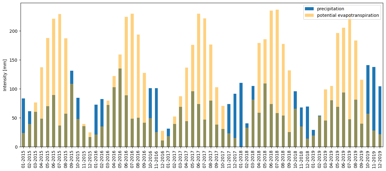
We evaluate the result on our location of interest:

# Transform the array into a pandas dataframe and sort the index.
meteo_df = ee_array_to_df(meteo_arr, ["pr", "pet"]).sort_index()

# Data visualization
fig, ax = plt.subplots(figsize=(15, 6))

# Barplot associated with precipitations.
meteo_df["pr"].plot(kind="bar", ax=ax, label="precipitation")

# Barplot associated with potential evapotranspiration.
meteo_df["pet"].plot(
    kind="bar", ax=ax, label="potential evapotranspiration", color="orange", alpha=0.5
)

# Add a legend.
ax.legend()

# Add some x/y-labels properties.
ax.set_ylabel("Intensity [mm]")
ax.set_xlabel(None)

# Define the date format and shape of x-labels.
x_labels = meteo_df.index.strftime("%m-%Y")
ax.set_xticklabels(x_labels, rotation=90, fontsize=10)

plt.show()

Implementation of the TM procedure

Description

Some additional definitions are needed to formalize the Thornthwaite-Mather procedure. The following definitions are given in accordance with Allen et al. (1998) (the document can be downloaded here):

where:

• \(TAW\): the total available soil water in the root zone [\(mm\)],
• \(\theta_{FC}\): the water content at the field capacity [\(m^{3} m^{-3}\)],
• \(\theta_{WP}\): the water content at wilting point [\(m^{3} m^{-3}\)],
• \(Z_{r}\): the rooting depth [\(m\)],

Typical values of \(\theta_{FC}\) and \(\theta_{WP}\) for different soil types are given in Table 19 of Allen et al. (1998).

The readily available water (\(RAW\)) is given by \(RAW = p \times TAW\), where \(p\) is the average fraction of \(TAW\) that can be depleted from the root zone before moisture stress (ranging between 0 to 1). This quantity is also noted \(ST_{FC}\) which is the available water stored at field capacity in the root zone.

Ranges of maximum effective rooting depth \(Z_{r}\), and soil water depletion fraction for no stress \(p\), for common crops are given in the Table 22 of Allen et al. (1998). In addition, a global effective plant rooting depth dataset is provided by Yang et al. (2016) with a resolution of 0.5° by 0.5° (see the paper here and the dataset here).

According to this global dataset, the effective rooting depth around our region of interest (France) can reasonably assumed to \(Z_{r} = 0.5\). Additionally, the parameter \(p\) is also assumed constant and equal to and \(p = 0.5\) which is in line with common values described in Table 22 of Allen et al. (1998).

zr = ee.Image(0.5)
p = ee.Image(0.5)

In the following, we also consider an averaged value between reference depths of the water content at wilting point and field capacity:

def olm_prop_mean(olm_image, band_output_name):
    """
    This function calculates an averaged value of
    soil properties between reference depths.
    """
    mean_image = olm_image.expression(
        "(b0 + b10 + b30 + b60 + b100 + b200) / 6",
        {
            "b0": olm_image.select("b0"),
            "b10": olm_image.select("b10"),
            "b30": olm_image.select("b30"),
            "b60": olm_image.select("b60"),
            "b100": olm_image.select("b100"),
            "b200": olm_image.select("b200"),
        },
    ).rename(band_output_name)

    return mean_image


# Apply the function to field capacity and wilting point.
fcm = olm_prop_mean(field_capacity, "fc_mean")
wpm = olm_prop_mean(wilting_point, "wp_mean")

# Calculate the theoretical available water.
taw = (
    (fcm.select("fc_mean").subtract(wpm.select("wp_mean"))).multiply(1000).multiply(zr)
)

# Calculate the stored water at the field capacity.
stfc = taw.multiply(p)

The Thornthwaite-Mather procedure used to estimate groundwater recharge is explicitly described by Steenhuis and Van der Molen (1985). This procedure uses monthly sums of potential evaporation, cumulative precipitation, and the moisture status of the soil which is calculated iteratively. The moisture status of the soils depends on the accumulated potential water loss (\(APWL\)). This parameter is calculated depending on whether the potential evaporation is greater than or less than the cumulative precipitation. The procedure reads as follow:

Case 1: potential evapotranspiration is higher than precipitation.

In that case, \(PET>P\) and \(APWL_{m}\) is incremented as follows: \(APWL_{m} = APWL_{m - 1} + (PET_{m} - P_{m})\) where:

• \(APWL_{m}\) (respectively \(APWL_{m - 1}\)) represents the accumulated potential water loss for the month \(m\) (respectively at the previous month \(m - 1\))
• \(PET_{m}\) the cumulative potential evapotranspiration at month \(m\),
• \(P_{m}\) the cumulative precipitation at month \(m\),

and the relationship between \(APWL\) and the amount of water stored in the root zone for the month \(m\) is expressed as: \(ST_{m} = ST_{FC} \times [\textrm{exp}(-APWL_{m}/ST_{FC})]\) where \(ST_{m}\) is the available water stored in the root zone for the month \(m\).

Case 2: potential evapotranspiration is lower than precipitation.

In that case, \(PET<P\) and \(ST_{m}\) is incremented as follows: \(ST_{m} = ST_{m-1} + (P_{m} - PET_{m})\).

Case 2.1: the storage \(ST_{m}\) is higher than the water stored at the field capacity.

If \(ST_{m} > ST_{FC}\) the recharge is calculated as: $$R_{m} = ST_{m} - ST_{FC} + P_{m} - PET_{m}$$

In addition, the water stored at the end of the month \(m\) becomes equal to \(ST_{FC}\) and \(APWL_{m}\) is set equal to zero.

Case 2.2: the storage \(ST_{m}\) is less than or equal to the water stored at the field capacity.

If \(ST_{m} <= ST_{FC}\), \(APWL_{m}\) is implemented as follows: \(APWL_{m} = - ST_{FC} \times \textrm{ln}(ST_{m}/ST_{FC})\), and no percolation occurs.

Initialization

The initial time of the calculation is defined according to the first date of the meteorological collection:

# Define the initial time (time0) according to the start of the collection.
time0 = meteo.first().get("system:time_start")

Then, we initialize the calculation with an ee.Image where all bands associated to the hydric state of the soil are set equal to ee.Image(0), except for the initial storage which is considered to be equal to the water content at field capacity, meaning that \(ST_{0} = ST_{FC}\).

# Initialize all bands describing the hydric state of the soil.
# Do not forget to cast the type of the data with a .float().
# Initial recharge.
initial_rech = ee.Image(0).set("system:time_start", time0).select([0], ["rech"]).float()

# Initialization of APWL.
initial_apwl = ee.Image(0).set("system:time_start", time0).select([0], ["apwl"]).float()

# Initialization of ST.
initial_st = stfc.set("system:time_start", time0).select([0], ["st"]).float()

# Initialization of precipitation.
initial_pr = ee.Image(0).set("system:time_start", time0).select([0], ["pr"]).float()

# Initialization of potential evapotranspiration.
initial_pet = ee.Image(0).set("system:time_start", time0).select([0], ["pet"]).float()

We combine all these bands into one ee.Image adding new bands to the first using the ee.Image.addBands method:

initial_image = initial_rech.addBands(
    ee.Image([initial_apwl, initial_st, initial_pr, initial_pet])
)

We also initialize a list in which new images will be added after each iteration. We create this server-side list using the ee.List method.

image_list = ee.List([initial_image])

Iteration over an ee.ImageCollection

The procedure is implemented by means of the ee.ImageCollection.iterate method, which applies a user-supplied function to each element of a collection. For each time step, groundwater recharge is calculated using the recharge_calculator considering the previous hydric state of the soil and current meteorological conditions.

Of course, considering the TM description, several cases must be distinguished to calculate groundwater recharge. The distinction is made by the definition of binary layers with different logical operations. It allows specific calculations to be applied in areas where a given condition is true using the ee.Image.where method.

The function we apply to each element of the meteorological dataset to calculate groundwater recharge is defined as follows.

def recharge_calculator(image, image_list):
    """
    Contains operations made at each iteration.
    """
    # Determine the date of the current ee.Image of the collection.
    localdate = image.date().millis()

    # Import previous image stored in the list.
    prev_im = ee.Image(ee.List(image_list).get(-1))

    # Import previous APWL and ST.
    prev_apwl = prev_im.select("apwl")
    prev_st = prev_im.select("st")

    # Import current precipitation and evapotranspiration.
    pr_im = image.select("pr")
    pet_im = image.select("pet")

    # Initialize the new bands associated with recharge, apwl and st.
    # DO NOT FORGET TO CAST THE TYPE WITH .float().
    new_rech = (
        ee.Image(0)
        .set("system:time_start", localdate)
        .select([0], ["rech"])
        .float()
    )

    new_apwl = (
        ee.Image(0)
        .set("system:time_start", localdate)
        .select([0], ["apwl"])
        .float()
    )

    new_st = (
        prev_st.set("system:time_start", localdate).select([0], ["st"]).float()
    )

    # Calculate bands depending on the situation using binary layers with
    # logical operations.

    # CASE 1.
    # Define zone1: the area where PET > P.
    zone1 = pet_im.gt(pr_im)

    # Calculation of APWL in zone 1.
    zone1_apwl = prev_apwl.add(pet_im.subtract(pr_im)).rename("apwl")
    # Implementation of zone 1 values for APWL.
    new_apwl = new_apwl.where(zone1, zone1_apwl)

    # Calculate ST in zone 1.
    zone1_st = stfc.multiply(
        ee.Image.exp(zone1_apwl.divide(stfc).multiply(-1))
    ).rename("st")
    # Implement ST in zone 1.
    new_st = new_st.where(zone1, zone1_st)

    # CASE 2.
    # Define zone2: the area where PET <= P.
    zone2 = pet_im.lte(pr_im)

    # Calculate ST in zone 2.
    zone2_st = prev_st.add(pr_im).subtract(pet_im).rename("st")
    # Implement ST in zone 2.
    new_st = new_st.where(zone2, zone2_st)

    # CASE 2.1.
    # Define zone21: the area where PET <= P and ST >= STfc.
    zone21 = zone2.And(zone2_st.gte(stfc))

    # Calculate recharge in zone 21.
    zone21_re = zone2_st.subtract(stfc).rename("rech")
    # Implement recharge in zone 21.
    new_rech = new_rech.where(zone21, zone21_re)
    # Implement ST in zone 21.
    new_st = new_st.where(zone21, stfc)

    # CASE 2.2.
    # Define zone 22: the area where PET <= P and ST < STfc.
    zone22 = zone2.And(zone2_st.lt(stfc))

    # Calculate APWL in zone 22.
    zone22_apwl = (
        stfc.multiply(-1).multiply(ee.Image.log(zone2_st.divide(stfc))).rename("apwl")
    )
    # Implement APWL in zone 22.
    new_apwl = new_apwl.where(zone22, zone22_apwl)

    # Create a mask around area where recharge can effectively be calculated.
    # Where we have have PET, P, FCm, WPm (except urban areas, etc.).
    mask = pet_im.gte(0).And(pr_im.gte(0)).And(fcm.gte(0)).And(wpm.gte(0))

    # Apply the mask.
    new_rech = new_rech.updateMask(mask)

    # Add all Bands to our ee.Image.
    new_image = new_rech.addBands(ee.Image([new_apwl, new_st, pr_im, pet_im]))

    # Add the new ee.Image to the ee.List.
    return ee.List(image_list).add(new_image)

The TM procedure can now be applied to the meteorological ee.ImageCollection:

# Iterate the user-supplied function to the meteo collection.
rech_list = meteo.iterate(recharge_calculator, image_list)

# Remove the initial image from our list.
rech_list = ee.List(rech_list).remove(initial_image)

# Transform the list into an ee.ImageCollection.
rech_coll = ee.ImageCollection(rech_list)

Let's have a look at the result around the location of interest:

arr = rech_coll.getRegion(poi, scale).getInfo()
rdf = ee_array_to_df(arr, ["pr", "pet", "apwl", "st", "rech"]).sort_index()
rdf.head(12)

The result can be displayed in the form of a barplot as follows:

# Data visualization in the form of barplots.
fig, ax = plt.subplots(figsize=(15, 6))

# Barplot associated with precipitation.
rdf["pr"].plot(kind="bar", ax=ax, label="precipitation", alpha=0.5)

# Barplot associated with potential evapotranspiration.
rdf["pet"].plot(
    kind="bar", ax=ax, label="potential evapotranspiration", color="orange", alpha=0.2
)

# Barplot associated with groundwater recharge
rdf["rech"].plot(kind="bar", ax=ax, label="recharge", color="green", alpha=1)

# Add a legend.
ax.legend()

# Define x/y-labels properties.
ax.set_ylabel("Intensity [mm]")
ax.set_xlabel(None)

# Define the date format and shape of x-labels.
x_labels = rdf.index.strftime("%m-%Y")
ax.set_xticklabels(x_labels, rotation=90, fontsize=10)

plt.show()

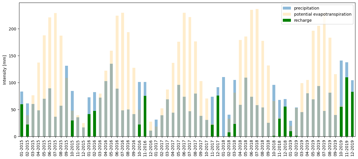
The result shows the distribution of precipitation, potential evapotranspiration, and groundwater recharge along the year. It shows that in our area of interest, groundwater recharge generally occurs from October to March. Even though a significant amount of precipitation occurs from April to September, evapotranspiration largely dominates because of high temperatures and sun exposure during these months. The result is that no percolation into aquifers occurs during this period.

Now the annual average recharge over the period of interest can be calculated. To do that, we resample the DataFrame we've just created:

# Resample the pandas dataframe on a yearly basis making the sum by year.
rdfy = rdf.resample("Y").sum()

# Calculate the mean value.
mean_recharge = rdfy["rech"].mean()

# Print the result.
print(
    "The mean annual recharge at our point of interest is", int(mean_recharge), "mm/an"
)

The mean annual recharge at our point of interest is 154 mm/an

/tmpfs/tmp/ipykernel_34716/1140476268.py:2: FutureWarning: 'Y' is deprecated and will be removed in a future version, please use 'YE' instead.
  rdfy = rdf.resample("Y").sum()

Groundwater recharge comparison between multiple places

We now may want to get local information about groundwater recharge and/or map this variable on an area of interest.

Let's define a function to get the local information based on the ee.ImageCollection we've just built:

def get_local_recharge(i_date, f_date, lon, lat, scale):
    """
    Returns a pandas df describing the cumulative groundwater
    recharge by month
    """
    # Define the location of interest with a point.
    poi = ee.Geometry.Point(lon, lat)

    # Evaluate the recharge around the location of interest.
    rarr = rech_coll.filterDate(i_date, f_date).getRegion(poi, scale).getInfo()

    # Transform the result into a pandas dataframe.
    rdf = ee_array_to_df(rarr, ["pr", "pet", "apwl", "st", "rech"]).sort_index()
    return rdf

We now use this function on a second point of interest located near the city of Montpellier (France). This city is located in the south of France, and precipitation and groundwater recharge are expected to be much lower than in the previous case.

# Define the second location of interest by longitude/latitude.
lon2 = 4.137152
lat2 = 43.626945

# Calculate the local recharge condition at this location.
rdf2 = get_local_recharge(i_date, f_date, lon2, lat2, scale)

# Resample the resulting pandas dataframe on a yearly basis (sum by year).
rdf2y = rdf2.resample("Y").sum()
rdf2y.head()

/tmpfs/tmp/ipykernel_34716/891754906.py:9: FutureWarning: 'Y' is deprecated and will be removed in a future version, please use 'YE' instead.
  rdf2y = rdf2.resample("Y").sum()

# Data Visualization
fig, ax = plt.subplots(figsize=(15, 6))
ax.axes.get_yaxis().set_visible(False)

# Define the x-label locations.
x = np.arange(len(rdfy))

# Define the bar width.
width = 0.25

# Bar plot associated to groundwater recharge at the 1st location of interest.
rect1 = ax.bar(
    x - width / 2, rdfy.rech, width, label="Lyon (France)", color="blue", alpha=0.5
)

# Bar plot associated to groundwater recharge at the 2nd location of interest.
rect2 = ax.bar(
    x + width / 2,
    rdf2y.rech,
    width,
    label="Montpellier (France)",
    color="red",
    alpha=0.5,
)

# Define a function to attach a label to each bar.
def autolabel_recharge(rects):
    """Attach a text label above each bar in *rects*, displaying its height."""
    for rect in rects:
        height = rect.get_height()
        ax.annotate(
            "{}".format(int(height)) + " mm",
            xy=(rect.get_x() + rect.get_width() / 2, height),
            xytext=(0, 3),  # 3 points vertical offset
            textcoords="offset points",
            ha="center",
            va="bottom",
            fontsize=8,
        )


autolabel_recharge(rect1)
autolabel_recharge(rect2)

# Calculate the averaged annual recharge at both locations of interest.
place1mean = int(rdfy["rech"].mean())
place2mean = int(rdf2y["rech"].mean())

# Add an horizontal line associated with averaged annual values (location 1).
ax.hlines(
    place1mean,
    xmin=min(x) - width,
    xmax=max(x) + width,
    color="blue",
    lw=0.5,
    label="average " + str(place1mean) + " mm/y",
    alpha=0.5,
)

# Add an horizontal line associated with averaged annual values (location 2).
ax.hlines(
    place2mean,
    xmin=min(x) - width,
    xmax=max(x) + width,
    color="red",
    lw=0.5,
    label="average " + str(place2mean) + " mm/y",
    alpha=0.5,
)

# Add a title.
ax.set_title("Groundwater recharge comparison between two places", fontsize=12)

# Define some x/y-axis properties.
ax.set_xticks(x)
x_labels = rdfy.index.year.tolist()
ax.set_xticklabels(x_labels, rotation=45, fontsize=10)

ax.spines["left"].set_visible(False)
ax.spines["right"].set_visible(False)
ax.spines["top"].set_visible(False)

# Shrink current axis's height by 10% on the bottom.
box = ax.get_position()
ax.set_position([box.x0, box.y0 + box.height * 0.1, box.width, box.height * 0.9])

# Add a legend below current axis.
ax.legend(
    loc="upper center", bbox_to_anchor=(0.5, -0.15), fancybox=True, shadow=True, ncol=2
)

plt.show()

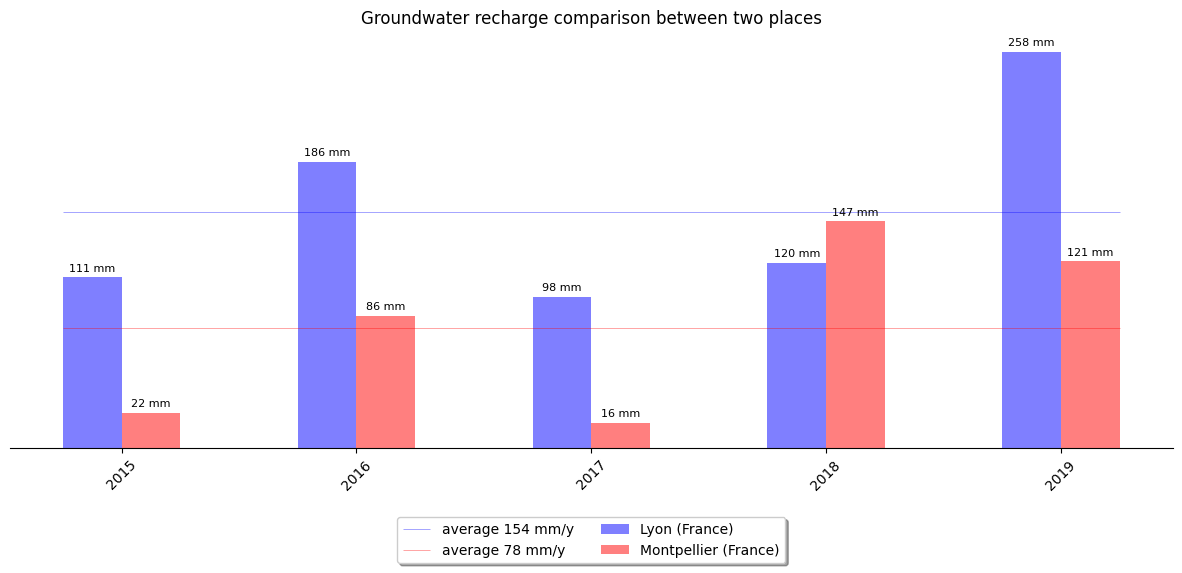
The result shows that the annual recharge in Lyon is almost twice as high as in the area of Montpellier. The result also shows a great variability of the annual recharge ranging from 98 mm/y to 258 mm/y in Lyon and from 16 mm/y to 147 mm/y in Montpellier.

Groundwater recharge map of France

To get a map of groundwater recharge around our region of interest, let's create a mean composite ee.Image based on our resulting ee.ImageCollection.

# Calculate the averaged annual recharge.
annual_rech = rech_coll.select("rech").mean().multiply(12)

# Calculate the average annual precipitation.
annual_pr = rech_coll.select("pr").mean().multiply(12)

# Get a feature collection of administrative boundaries.
countries = ee.FeatureCollection("FAO/GAUL/2015/level0").select("ADM0_NAME")

# Filter the feature collection to subset France.
france = countries.filter(ee.Filter.eq("ADM0_NAME", "France"))

# Clip the composite ee.Images around the region of interest.
rech_france = annual_rech.clip(france)
pr_france = annual_pr.clip(france)

And finally the map can be drawn.

# Create a folium map.
my_map = folium.Map(location=[lat, lon], zoom_start=6, zoom_control=False)

# Set visualization parameters for recharge.
rech_vis_params = {
    "bands": "rech",
    "min": 0,
    "max": 500,
    "opacity": 1,
    "palette": ["red", "orange", "yellow", "green", "blue", "purple"],
}

# Set visualization parameters for precipitation.
pr_vis_params = {
    "bands": "pr",
    "min": 500,
    "max": 1500,
    "opacity": 1,
    "palette": ["white", "blue"],
}

# Define a recharge colormap.
rech_colormap = cm.LinearColormap(
    colors=rech_vis_params["palette"],
    vmin=rech_vis_params["min"],
    vmax=rech_vis_params["max"],
)

# Define a precipitation colormap.
pr_colormap = cm.LinearColormap(
    colors=pr_vis_params["palette"],
    vmin=pr_vis_params["min"],
    vmax=pr_vis_params["max"],
)

# Caption of the recharge colormap.
rech_colormap.caption = "Average annual recharge rate (mm/year)"

# Caption of the precipitation colormap.
pr_colormap.caption = "Average annual precipitation rate (mm/year)"

# Add the precipitation composite to the map object.
my_map.add_ee_layer(pr_france, pr_vis_params, "Precipitation")

# Add the recharge composite to the map object.
my_map.add_ee_layer(rech_france, rech_vis_params, "Recharge")

# Add a marker at both locations of interest.
folium.Marker([lat, lon], popup="Area of Lyon").add_to(my_map)
folium.Marker([lat2, lon2], popup="Area of Montpellier").add_to(my_map)

# Add the colormaps to the map.
my_map.add_child(rech_colormap)
my_map.add_child(pr_colormap)

# Add a layer control panel to the map.
my_map.add_child(folium.LayerControl())

# Display the map.
display(my_map)

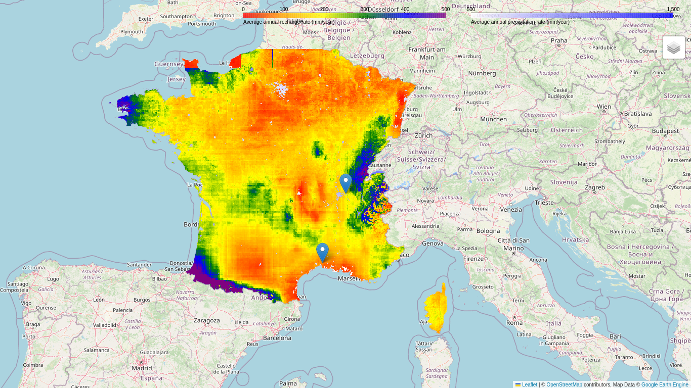
The resulting map represents the averaged annual precipitation and groundwater recharge rate in France over the period 2015-2019. Groundwater recharge is represented between 0 (red) to 500 mm/year (purple). Precipitation is represented between 500 (white) to 1500 mm/year (blue).

Please note the following points:

• The precipitation dataset used in this tutorial is not available over +/- 50 deg latitudes. That is why (1) the northern part of France is not covered by the precipitation/recharge, and (2) some anomalies/discontinuities can be observed near the boundary of the dataset.
• The procedure described in this tutorial does not consider the terrain slope which has a strong influence on runoff, especially in areas with significant relief. In these areas, groundwater recharge is overestimated because runoff is not considered.
• Snow cover has a more complex contribution to groundwater recharge than precipitation. This process is not taken into account in this tutorial. Hence, groundwater recharge is overestimated in areas where snow cover period is significant.
• The recharge calculation can be highly influenced by missing precipitation or potential evapotranspiration values. This issue is partially addressed by the dataset resampling procedure, but missing value can still exist and this point must be checked before considering that the calculated recharge is representative and reliable.

Bibliography

Allen RG, Pereira LS, Raes D, Smith M (1998). Crop evapotranspiration: guidelines for computing crop water requirements. Irrigation and Drainage Paper 56, FAO, Rome.

Saxton, K. E., & Rawls, W. J. (2006). Soil water characteristic estimates by texture and organic matter for hydrologic solutions. Soil science society of America Journal, 70(5), 1569-1578.

Steenhuis, T. S., & Van der Molen, W. H. (1986). The Thornthwaite-Mather procedure as a simple engineering method to predict recharge. Journal of Hydrology, 84(3-4), 221-229.

Thornthwaite, C. W., & Mather, J. R. (1957). Instructions and tables for computing potential evapotranspiration and the water balance. Publ. Climatol., 10(3).

Yang, Y., Donohue, R. J., & McVicar, T. R. (2016). Global estimation of effective plant rooting depth: Implications for hydrological modeling. Water Resources Research, 52(10), 8260-8276.

Acknowledgements

Thanks to Susanne Benz for precious advice.