Visualize Places Insights Data Dynamically with Looker Studio

Overview

This document describes how to build dynamic geospatial reports using Places Insights and Looker Studio. Unlock the value of your location data by empowering non-technical stakeholders to answer their own questions. This guide shows you how to turn static reports into interactive, heatmap-style tools for market analysis, without having to write SQL for every request. Enable access to complex location data, bridging the gap between data engineering and business intelligence.

Adopting this architectural pattern unlocks several key benefits:

• Visual Data Representation: Transforms Places Insights data into interactive maps and charts that immediately communicate spatial density and trends.
• Simplified Exploration without SQL: Enables team members, such as market analysts or real estate planners, to dynamically filter data using predefined parameters (e.g., changing "City" or "Time of Day" using dropdowns). They can explore the data without ever writing a single line of SQL.
• Seamless Collaboration: Standard Looker Studio sharing features allow you to securely distribute these interactive insights.

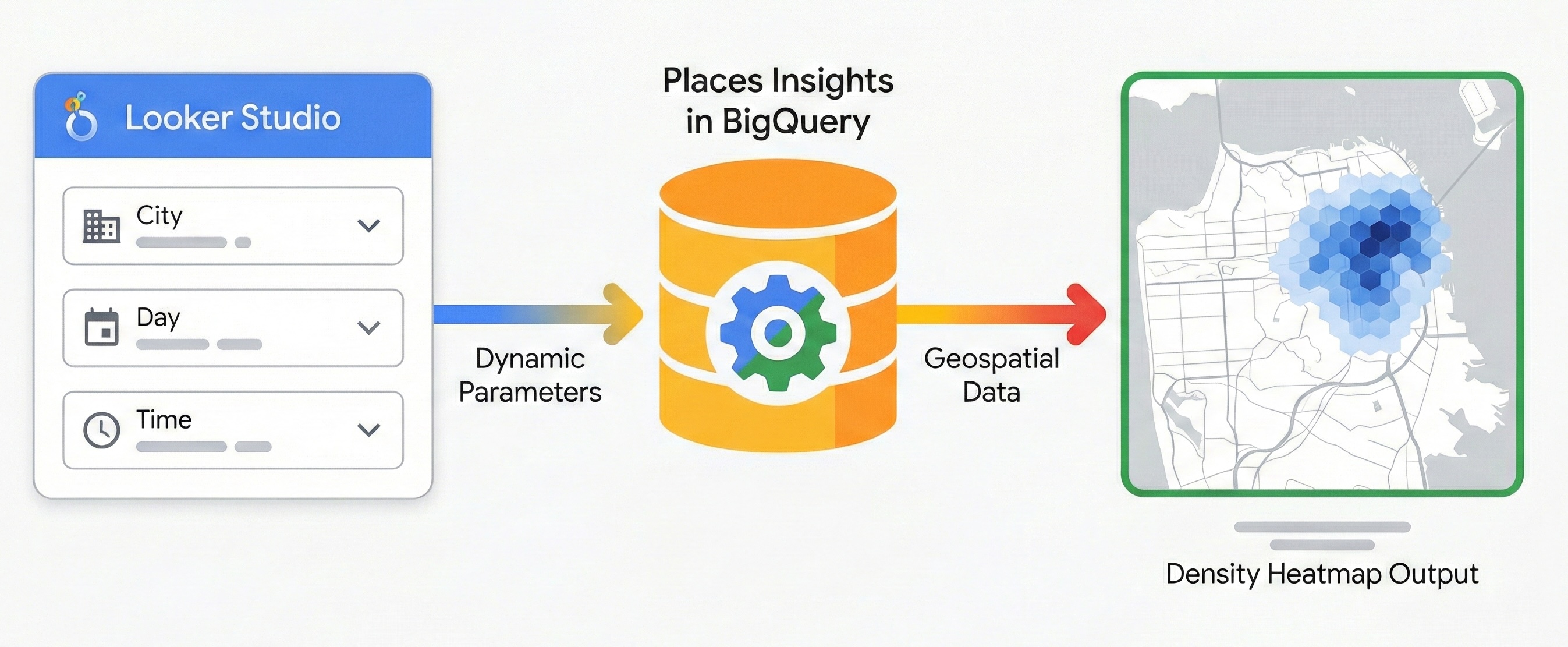
Solution Workflow

The following workflow establishes a performant reporting architecture. It moves from a static baseline to a fully dynamic application, ensuring data correctness before introducing complexity.

Prerequisites

Before you begin, follow these instructions to set up Places Insights. You will need access to Looker Studio, which is a no-cost tool.

Step 1: Establish a Static Geospatial Baseline

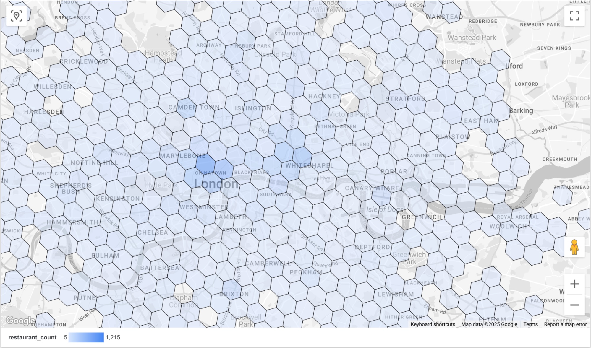
Before introducing interactivity, establish a base query and ensure it renders correctly in Looker Studio. Use Places Insights and BigQuery's geospatial capabilities to aggregate data into hexagonal grids using the H3 indexing system. This will produce a query output that can be used with Looker Studio's filled map cart type for visualization.

1.1 Connect Data

Use the following static query to establish the initial connection. It targets a fixed location (London) and category (Restaurants) to validate the data pipeline.

SELECT
  h3_index,
  `carto-os.carto.H3_BOUNDARY`(h3_index) AS h3_geo,
  restaurant_count
FROM (
  SELECT WITH AGGREGATION_THRESHOLD
    `carto-os.carto.H3_FROMGEOGPOINT`(point, 8) AS h3_index,
    COUNT(*) AS restaurant_count
  FROM
    -- Note: Change 'gb' to your target country code (e.g., 'us')
    `places_insights___gb.places`
  WHERE
    'London' IN UNNEST(locality_names)
    AND 'restaurant' IN UNNEST(types)
  GROUP BY
    h3_index
)
ORDER BY
  restaurant_count DESC;

Note on Spatial Aggregation

This query uses the public CARTO Spatial Extension (carto-os) available in BigQuery. The H3_FROMGEOGPOINT function converts specific location points into H3 cells, a system that divides the world into hexagonal grid cells.

We use this transformation because Looker Studio's Filled Map requires polygons (shapes) to render colors. By converting points into hexagonal shapes, we can visualize the density of businesses in a specific area, rather than plotting thousands of overlapping dots.

Note on Aggregation Threshold

All Places Insights queries require the WITH AGGREGATION_THRESHOLD clause. This privacy protection ensures that data is only returned if the aggregated count is 5 or higher.

In the context of this visualization, if a H3 grid cell contains fewer than 5 restaurants, that cell is omitted from the result set entirely and will appear empty on your map.

To implement this in Looker Studio:

1. Create a new Blank Report.
2. Select BigQuery as the data connector.
3. Choose CUSTOM QUERY from the left-hand menu and select your billing Project ID.
4. Paste the Static Base Query above into the editor.
5. Clear Use Legacy SQL, Enable date range, and Enable viewer email address parameters.
6. Click Add.

1.2 Configure Geospatial Visualization

Once the data is connected, configure Looker Studio to recognize the H3 boundary data correctly:

1. Add a Filled Map visualization to the report canvas, from the Add a chart menu.
2. Make sure that your h3_geo field, which contains the polygon geometry, is set to the Geospatial data type.
   1. Click the Edit data source (pencil) icon next to your connection name.
   2. If h3_geo is set to Text (ABC), use the drop-down menu to select Geo > Geospatial,
   3. Click Done.
3. Map the h3_index field to Location (acting as the unique identifier).
4. Map the h3_geo field to Geospatial Field (acting as the polygon geometry).
5. Map the restaurant_count field to Color metric.

This will render a map of restaurant density by H3 cell. The darker blue (default color option) indicates a cell with a higher restaurant count.

Step 2: Implement Dynamic Parameters

To make the report interactive, we will add controls to the report that allow the user to select from the following options:

• Locality: Controls the city the report focuses on.
• Day of the week: Filters places based on the day they are open, leveraging the regular_opening_hours record in the schema.
• Hour of the day: Filters places based on their operational hours by comparing against the start_time and end_time fields.

To achieve this, you will pass user-selected parameters directly into a modified Places Insights query at runtime. In Looker Studio's data source editor, you must explicitly define these parameters as typed variables.

In Looker Studio, select the Resource menu, then click Manage added data sources. Within the panel that appears, select EDIT against the BigQuery Custom SQL data source we added earlier.

Within the Edit Connection window, select ADD A PARAMETER. We are going to add three parameters, with the values below.

Example configuration for the p_hour_of_day parameter.

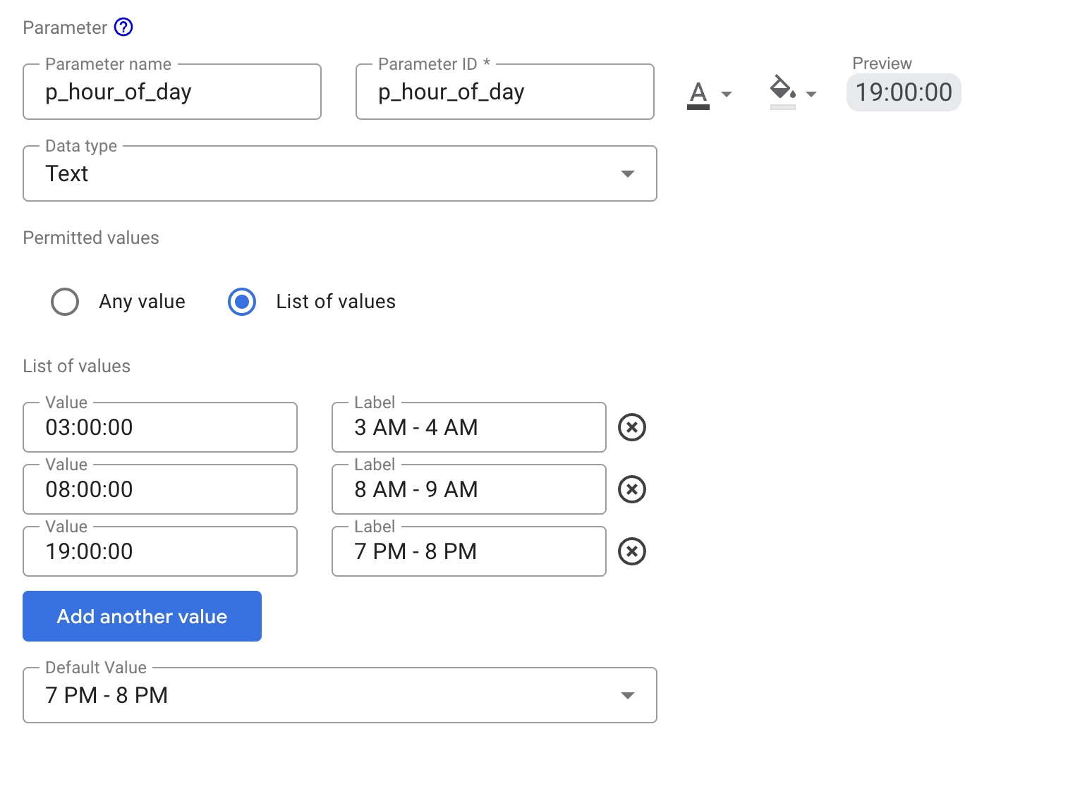
For the p_hour_of_day parameter, pay close attention to the Value column. Because the SQL query uses CAST(@p_hour_of_day AS TIME), the values passed from Looker Studio must be in strict HH:MM:SS format (24-hour clock).

Once you have set up and saved all three parameters, modify your BigQuery Custom SQL connection to reference these variables using the @ syntax.

This is done by clicking Edit Connection, and pasting in the below modified query:

SELECT
  h3_index,
  `carto-os.carto.H3_BOUNDARY`(h3_index) AS h3_geo,
  restaurant_count
FROM (
  SELECT WITH AGGREGATION_THRESHOLD
    `carto-os.carto.H3_FROMGEOGPOINT`(point, 8) AS h3_index,
    COUNT(*) AS restaurant_count
  FROM
    `places_insights___gb.places`
  WHERE
    -- Dynamic locality filter based on parameter
    @p_locality IN UNNEST(locality_names)
    AND 'restaurant' IN UNNEST(types)
    AND business_status = 'OPERATIONAL'
    AND EXISTS (
      SELECT 1
      FROM UNNEST(
        CASE @p_day_of_week
          WHEN 'monday' THEN regular_opening_hours.monday
          WHEN 'tuesday' THEN regular_opening_hours.tuesday
          WHEN 'wednesday' THEN regular_opening_hours.wednesday
          WHEN 'thursday' THEN regular_opening_hours.thursday
          WHEN 'friday' THEN regular_opening_hours.friday
          WHEN 'saturday' THEN regular_opening_hours.saturday
          WHEN 'sunday' THEN regular_opening_hours.sunday
        END
      ) AS hours
      WHERE hours.start_time <= CAST(@p_hour_of_day AS TIME)
        AND hours.end_time >= TIME_ADD(CAST(@p_hour_of_day AS TIME), INTERVAL 1 HOUR)
    )
  GROUP BY
    h3_index
)
ORDER BY
  restaurant_count DESC;

Click Reconnect to save the edit. In the modified query, note the new variables such as @p_hour_of_day, which correlate to the parameter names we just set up.

Return to the report canvas to expose these parameters to the end user:

1. Add three Drop-down list controls to your report.
2. For each control, set the Control field to correspond to your newly created parameters:
   • Control 1: p_locality
   • Control 2: p_day_of_week
   • Control 3: p_hour_of_day

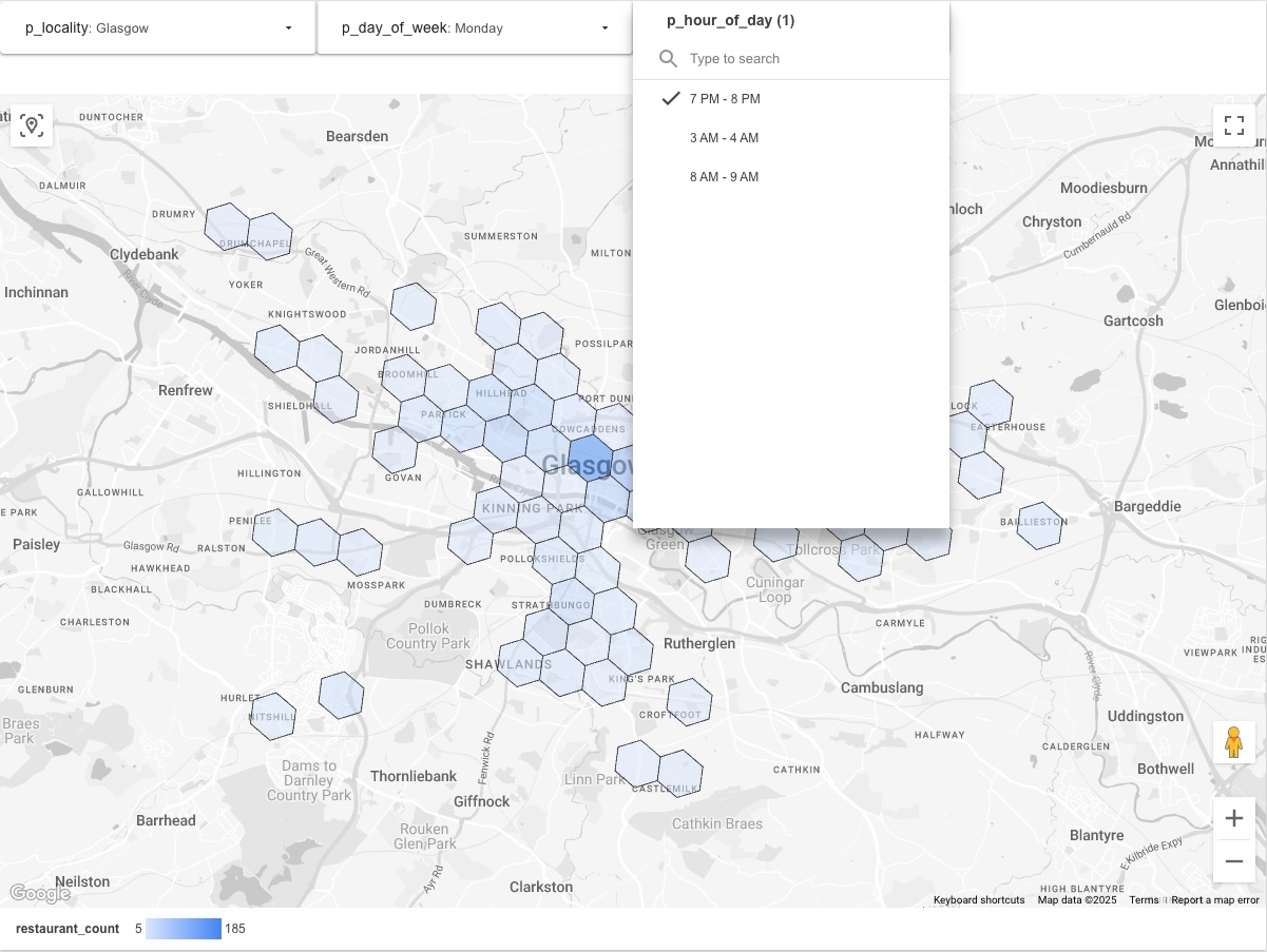
Your final report should look like the following. Changing a value in one of the drop-down controls will trigger Looker Studio to fetch the requested data from Places Insights before visualizing on the map.

Step 3: Share the results

Use the sharing tool built into Looker Studio to share the report. This will allow viewers to dynamically update the visualization based on the parameters they select from your drop-down lists.

Conclusion

This pattern creates a scalable, interactive reporting tool that leverages BigQuery's computational power to serve aggregated Places Insights data to Looker Studio. This architecture avoids the pitfalls of trying to visualize massive raw datasets and provides end-users with the flexibility to explore data across different dimensions, like time, location, and business type, in near real-time. This is a powerful tool to give your non-technical stakeholders flexibility to explore the data.

Next Steps

Explore other variations of dynamic reports by parameterizing different parts of the Places Insights schema:

• Dynamic Competitor Analysis: Create a parameter for brand names to allow users to instantly switch the heatmap between different competitors to see their relative saturation in a market. See About Places Insights data for brand data availability.
• Interactive Site Selection: Add parameters for price_level (e.g., 'Moderate' versus 'Expensive') and minimum rating to allow real estate teams to dynamically filter for areas that match specific demographic profiles.
• Custom Catchment Areas: Instead of filtering by city name, allow users to define custom study areas.
  • Radius-based: Create three numeric parameters: p_latitude, p_longitude, and p_radius_meters. Coordinates can be obtained from Google Maps Platform APIs, including the Geocoding API. In your query, inject these into the ST_DWITHIN function:
    • ST_DWITHIN(point, ST_GEOGPOINT(@p_longitude, @p_latitude), @p_radius_meters)
  • Polygon-based: For complex custom shapes (like sales territories), users cannot easily input geometry text. Instead, create a lookup table in BigQuery containing your shape geometries and a friendly name (e.g., "Zone A"). Create a text parameter p_zone_name in Looker Studio to let users select the zone, and use a subquery to retrieve the geometry for the ST_CONTAINS function.

Contributors

• David Szajngarten | Developer Relations Engineer
• Henrik Valve | DevX Engineer