如需从 Image(栅格)转换为 FeatureCollection(矢量)数据类型,请使用 image.reduceToVectors()。这是 Earth Engine 中矢量化的主要机制,对于生成要输入到其他类型的 reducer 的区域非常有用。reduceToVectors() 方法会在连接的像素的均匀组的边界处创建多边形边缘(可选替换为质心或边界框)。
例如,请考虑 2012 年日本的夜灯图片。让夜灯数字编号充当开发强度的代理。使用夜灯上的任意阈值定义区域,将区域合并为单波段图像,使用 reduceToVectors() 将区域矢量化:
Code Editor (JavaScript)
// Load a Japan boundary from the Large Scale International Boundary dataset.
var japan = ee.FeatureCollection('USDOS/LSIB_SIMPLE/2017')
  .filter(ee.Filter.eq('country_na', 'Japan'));

// Load a 2012 nightlights image, clipped to the Japan border.
var nl2012 = ee.Image('NOAA/DMSP-OLS/NIGHTTIME_LIGHTS/F182012')
  .select('stable_lights')
  .clipToCollection(japan);

// Define arbitrary thresholds on the 6-bit nightlights image.
var zones = nl2012.gt(30).add(nl2012.gt(55)).add(nl2012.gt(62));
zones = zones.updateMask(zones.neq(0));

// Convert the zones of the thresholded nightlights to vectors.
var vectors = zones.addBands(nl2012).reduceToVectors({
  geometry: japan,
  crs: nl2012.projection(),
  scale: 1000,
  geometryType: 'polygon',
  eightConnected: false,
  labelProperty: 'zone',
  reducer: ee.Reducer.mean()
});

// Display the thresholds.
Map.setCenter(139.6225, 35.712, 9);
Map.addLayer(zones, {min: 1, max: 3, palette: ['0000FF', '00FF00', 'FF0000']}, 'raster');

// Make a display image for the vectors, add it to the map.
var display = ee.Image(0).updateMask(0).paint(vectors, '000000', 3);
Map.addLayer(display, {palette: '000000'}, 'vectors');
import ee
import geemap.core as geemap
Colab (Python)
# Load a Japan boundary from the Large Scale International Boundary dataset.
japan = ee.FeatureCollection('USDOS/LSIB_SIMPLE/2017').filter(
    ee.Filter.eq('country_na', 'Japan')
)

# Load a 2012 nightlights image, clipped to the Japan border.
nl_2012 = (
    ee.Image('NOAA/DMSP-OLS/NIGHTTIME_LIGHTS/F182012')
    .select('stable_lights')
    .clipToCollection(japan)
)

# Define arbitrary thresholds on the 6-bit nightlights image.
zones = nl_2012.gt(30).add(nl_2012.gt(55)).add(nl_2012.gt(62))
zones = zones.updateMask(zones.neq(0))

# Convert the zones of the thresholded nightlights to vectors.
vectors = zones.addBands(nl_2012).reduceToVectors(
    geometry=japan,
    crs=nl_2012.projection(),
    scale=1000,
    geometryType='polygon',
    eightConnected=False,
    labelProperty='zone',
    reducer=ee.Reducer.mean(),
)

# Display the thresholds.
m = geemap.Map()
m.set_center(139.6225, 35.712, 9)
m.add_layer(
    zones,
    {'min': 1, 'max': 3, 'palette': ['0000FF', '00FF00', 'FF0000']},
    'raster',
)

# Make a display image for the vectors, add it to the map.
display_image = ee.Image(0).updateMask(0).paint(vectors, '000000', 3)
m.add_layer(display_image, {'palette': '000000'}, 'vectors')
m
请注意,输入中的第一个波段用于识别均匀区域,其余波段会根据提供的 reducer 进行缩减,其输出会作为属性添加到生成的矢量中。geometry 参数指定应在哪个范围内创建矢量。一般而言,建议您指定用于创建矢量的最小区域。最好也指定 scale 和 crs,以免产生歧义。输出类型为 ‘polygon’,其中多边形由四相邻邻区的同质区域组成(即 eightConnected 为 false)。最后两个参数 labelProperty 和 reducer 分别指定输出多边形应分别接收包含区域标签和夜间灯带平均值的属性。
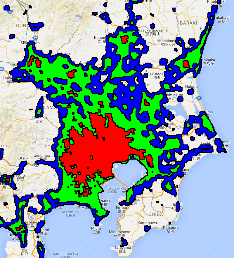
映射结果应如下图 1 所示的东京地区。 检查输出多边形后发现,由于指定了平均值归约器,因此每个多边形都有一个属性,用于存储区域的标签 ({1, 2, 3}) 和夜间灯带的平均值。