“水体出现变化强度”数据层可衡量地表水在两个时间段(1984 年至 1999 年和 2000 年至 2015 年)之间的变化情况。该层会对两个时间段中同源的月份对之间的变化求平均值。如需详细了解此图层,请参阅 数据用户指南(第 2 版) 。
本教程的这一部分将:
- 添加一个样式化地图图层,用于直观呈现水域出现强度变化,以及
- 使用直方图总结指定感兴趣区域内的变化强度。
可视化
与水体出现图层类似,我们将首先向地图添加出现变化强度的基本可视化效果,然后再对其进行改进。系统会以两种方式提供出现次数变化强度,即绝对值和归一化值。在本教程中,我们将使用绝对值。 首先,从 GSW 映像中选择绝对出现次数变化强度层:
代码编辑器 (JavaScript)
var change = gsw.select("change_abs");
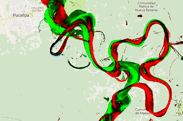
在代码的“常量”部分中,添加一条语句,用于创建一个新变量来定义图层的样式设置方式。此样式以红色/绿色显示地表水出现次数减少/增加的区域。地表水出现频率相对不变的区域以黑色显示。
代码编辑器 (JavaScript)
var VIS_CHANGE = {
    min:-50,
    max:50,
    palette: ['red', 'black', 'limegreen']
};
在“地图图层”部分的代码末尾,添加一条向地图添加新图层的语句。
代码编辑器 (JavaScript)
Map.setCenter(-74.4557, -8.4289, 11);  // Ucayali River, Peru
Map.addLayer({
  eeObject: change,
  visParams: VIS_CHANGE,
  name: 'occurrence change intensity'
});
总结感兴趣区域内的变化
在本部分中,我们将总结指定感兴趣区域内的变化量。如需指定感兴趣的区域,请点击多边形绘制工具,该工具是 几何图形工具之一。 这会创建一个新的“几何图形导入”图层,默认名称为“geometry”。如需更改名称,请点击图层名称右侧的齿轮图标。(请注意,您可能需要将光标放在图层名称上才能显示该名称。)
将图层名称更改为 roi(表示感兴趣区域或投资回报率)。然后,我们可以点击地图上的一系列点,以定义多边形感兴趣区域。
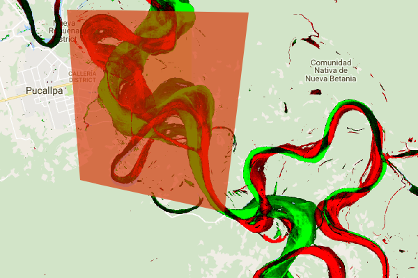
现在,我们已经定义了感兴趣区域并将其存储在一个变量中,接下来可以使用该变量来计算投资回报率的变化强度直方图。将以下代码添加到脚本的“计算”部分。
代码编辑器 (JavaScript)
// Calculate a change intensity for the region of interest.
var histogram = change.reduceRegion({
  reducer: ee.Reducer.histogram(),
  geometry: roi,
  scale: 30,
  bestEffort: true,
});
print(histogram);
第一个语句用于计算投资回报率 (ROI) 内出现次数变化强度值的直方图,并以 30 米的比例进行采样。第二个函数会将生成的对象输出到代码编辑器控制台标签页。您可以展开对象树,查看直方图区桶的值。 虽然有数值数据,但有更好的方式来直观呈现结果。
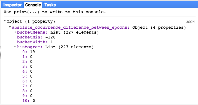
为了改进这一点,我们可以改为生成直方图。将定义直方图对象的语句替换为以下语句:
代码编辑器 (JavaScript)
// Generate a histogram object and print it to the console tab.
var histogram = ui.Chart.image.histogram({
  image: change,
  region: roi,
  scale: 30,
  minBucketWidth: 10
});
histogram.setOptions({
  title: 'Histogram of surface water change intensity.'
});
这些语句会创建一个直方图对象,该对象会替换控制台标签页中的直方图对象树。图表方法包含多个实参,包括 scale(用于定义感兴趣区域的采样空间尺度,以米为单位)和 minBucketWidth(用于控制直方图分桶的宽度)。
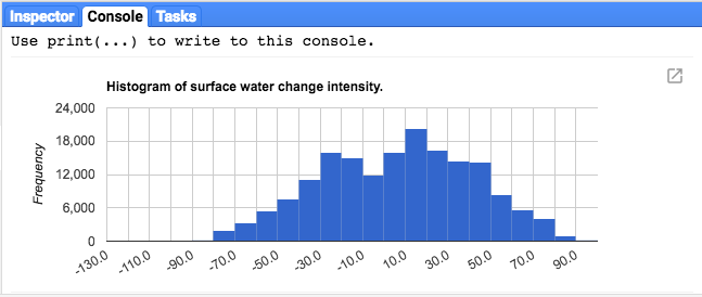
您可以将光标悬停在直方图条柱上,以互动方式探索图表值。
最终脚本
此部分的完整脚本如下所示。请注意,该脚本包含用于定义多边形几何图形 (roi) 的语句,这与您使用代码编辑器的几何图形工具创建的几何图形类似。
代码编辑器 (JavaScript)
//////////////////////////////////////////////////////////////
// Asset List
//////////////////////////////////////////////////////////////

var gsw = ee.Image('JRC/GSW1_0/GlobalSurfaceWater');
var occurrence = gsw.select('occurrence');
var change = gsw.select("change_abs");
var roi = /* color: 0B4A8B */ee.Geometry.Polygon(
        [[[-74.17213, -8.65569],
          [-74.17419, -8.39222],
          [-74.38362, -8.36980],
          [-74.43031, -8.61293]]]);

//////////////////////////////////////////////////////////////
// Constants
//////////////////////////////////////////////////////////////

var VIS_OCCURRENCE = {
    min:0,
    max:100,
    palette: ['red', 'blue']
};
var VIS_CHANGE = {
    min:-50,
    max:50,
    palette: ['red', 'black', 'limegreen']
};
var VIS_WATER_MASK = {
  palette: ['white', 'black']
};

//////////////////////////////////////////////////////////////
// Calculations
//////////////////////////////////////////////////////////////

// Create a water mask layer, and set the image mask so that non-water areas are transparent.
var water_mask = occurrence.gt(90).mask(1);

// Generate a histogram object and print it to the console tab.
var histogram = ui.Chart.image.histogram({
  image: change,
  region: roi,
  scale: 30,
  minBucketWidth: 10
});
histogram.setOptions({
  title: 'Histogram of surface water change intensity.'
});
print(histogram);

//////////////////////////////////////////////////////////////
// Initialize Map Location
//////////////////////////////////////////////////////////////

// Uncomment one of the following statements to center the map on
// a particular location.
// Map.setCenter(-90.162, 29.8597, 10);   // New Orleans, USA
// Map.setCenter(-114.9774, 31.9254, 10); // Mouth of the Colorado River, Mexico
// Map.setCenter(-111.1871, 37.0963, 11); // Lake Powell, USA
// Map.setCenter(149.412, -35.0789, 11);  // Lake George, Australia
// Map.setCenter(105.26, 11.2134, 9);     // Mekong River Basin, SouthEast Asia
// Map.setCenter(90.6743, 22.7382, 10);   // Meghna River, Bangladesh
// Map.setCenter(81.2714, 16.5079, 11);   // Godavari River Basin Irrigation Project, India
// Map.setCenter(14.7035, 52.0985, 12);   // River Oder, Germany & Poland
// Map.setCenter(-59.1696, -33.8111, 9);  // Buenos Aires, Argentina\
Map.setCenter(-74.4557, -8.4289, 11);  // Ucayali River, Peru

//////////////////////////////////////////////////////////////
// Map Layers
//////////////////////////////////////////////////////////////

Map.addLayer({
  eeObject: water_mask,
  visParams: VIS_WATER_MASK,
  name: '90% occurrence water mask',
  shown: false
});
Map.addLayer({
  eeObject: occurrence.updateMask(occurrence.divide(100)),
  name: "Water Occurrence (1984-2015)",
  visParams: VIS_OCCURRENCE,
  shown: false
});
Map.addLayer({
  eeObject: change,
  visParams: VIS_CHANGE,
  name: 'occurrence change intensity'
});
在下一部分中,您将通过使用水体类别转变图层进一步探索水体随时间的变化。