Earth Engine 中的数组由数字列表和列表列表构成。嵌套程度决定了维度数。如需从一个简单且有意义的示例入手,请考虑以下使用 Landsat 8 平顶帽 (TC) 系数创建的 Array 示例(Baig 等人,2014 年):
Code Editor (JavaScript)
// Create an Array of Tasseled Cap coefficients.
var coefficients = ee.Array([
  [0.3029, 0.2786, 0.4733, 0.5599, 0.508, 0.1872],
  [-0.2941, -0.243, -0.5424, 0.7276, 0.0713, -0.1608],
  [0.1511, 0.1973, 0.3283, 0.3407, -0.7117, -0.4559],
  [-0.8239, 0.0849, 0.4396, -0.058, 0.2013, -0.2773],
  [-0.3294, 0.0557, 0.1056, 0.1855, -0.4349, 0.8085],
  [0.1079, -0.9023, 0.4119, 0.0575, -0.0259, 0.0252],
]);
import ee
import geemap.core as geemap
Colab (Python)
# Create an Array of Tasseled Cap coefficients.
coefficients = ee.Array([
    [0.3029, 0.2786, 0.4733, 0.5599, 0.508, 0.1872],
    [-0.2941, -0.243, -0.5424, 0.7276, 0.0713, -0.1608],
    [0.1511, 0.1973, 0.3283, 0.3407, -0.7117, -0.4559],
    [-0.8239, 0.0849, 0.4396, -0.058, 0.2013, -0.2773],
    [-0.3294, 0.0557, 0.1056, 0.1855, -0.4349, 0.8085],
    [0.1079, -0.9023, 0.4119, 0.0575, -0.0259, 0.0252],
])
使用 length() 确认这是一个 6x6 的二维数组,它将返回每个轴的长度:
Code Editor (JavaScript)
// Print the dimensions.
print(coefficients.length()); //    [6,6]
import ee
import geemap.core as geemap
Colab (Python)
# Print the dimensions.
display(coefficients.length())  #    [6,6]
下表展示了矩阵条目沿着 0 轴和 1 轴的排列方式:
| 1 轴 -> | |||||||
|---|---|---|---|---|---|---|---|
| 0 | 1 | 2 | 3 | 4 | 5 | ||
| 0 | 0.3029 | 0.2786 | 0.4733 | 0.5599 | 0.508 | 0.1872 | |
| 1 | -0.2941 | -0.243 | -0.5424 | 0.7276 | 0.0713 | -0.1608 | |
| 0 轴 | 2 | 0.1511 | 0.1973 | 0.3283 | 0.3407 | -0.7117 | -0.4559 |
| 3 | -0.8239 | 0.0849 | 0.4396 | -0.058 | 0.2013 | -0.2773 | |
| 4 | -0.3294 | 0.0557 | 0.1056 | 0.1855 | -0.4349 | 0.8085 | |
| 5 | 0.1079 | -0.9023 | 0.4119 | 0.0575 | -0.0259 | 0.0252 | |
表格左侧的索引表示沿 0 轴的位置。0 轴上每个列表中的第 n 个元素位于 1 轴的第 n 个位置。例如,数组坐标 [3,1] 对应的条目为 0.0849。假设“绿度”是感兴趣的 TC 组成部分。您可以使用 slice() 获取绿度子矩阵:
Code Editor (JavaScript)
// Get the 1x6 greenness slice, display it.
var greenness = coefficients.slice({axis: 0, start: 1, end: 2, step: 1});
print(greenness);
import ee
import geemap.core as geemap
Colab (Python)
# Get the 1x6 greenness slice, display it.
greenness = coefficients.slice(axis=0, start=1, end=2, step=1)
display(greenness)
二维绿度矩阵应如下所示:
[[-0.2941,-0.243,-0.5424,0.7276,0.0713,-0.1608]]
请注意,slice() 的 start 和 end 参数对应于表格中显示的 0 轴索引(start 是包含边界,end 是不含边界)。
数组图片
如需获取绿度图像,请将 Landsat 8 图像的波段与绿度矩阵进行矩阵乘法。为此,请先将多波段 Landsat 图像转换为“数组图像”,其中每个像素都是波段值的 Array。例如:
Code Editor (JavaScript)
// Load a Landsat 8 image, select the bands of interest.
var image = ee.Image('LANDSAT/LC08/C02/T1_TOA/LC08_044034_20140318')
  .select(['B2', 'B3', 'B4', 'B5', 'B6', 'B7']);

// Make an Array Image, with a 1-D Array per pixel.
var arrayImage1D = image.toArray();

// Make an Array Image with a 2-D Array per pixel, 6x1.
var arrayImage2D = arrayImage1D.toArray(1);
import ee
import geemap.core as geemap
Colab (Python)
# Load a Landsat 8 image, select the bands of interest.
image = ee.Image('LANDSAT/LC08/C02/T1_TOA/LC08_044034_20140318').select(
    ['B2', 'B3', 'B4', 'B5', 'B6', 'B7']
)

# Make an Array Image, with a 1-D Array per pixel.
array_image_1d = image.toArray()

# Make an Array Image with a 2-D Array per pixel, 6x1.
array_image_2d = array_image_1d.toArray(1)
在此示例中,请注意 toArray() 会将 image 转换为数组图像,其中每个像素都是一个 1 维矢量,其条目对应于 image 波段中相应位置的 6 个值。以这种方式创建的一维向量数组图像没有二维形状的概念。如需执行仅限 2D 的操作(例如矩阵乘法),请使用 toArray(1) 将其转换为每个像素的 2D 数组图片。二维数组图像的每个像素中,都有一个 6x1 的波段值矩阵。为此,请考虑以下示例:
Code Editor (JavaScript)
var array1D = ee.Array([1, 2, 3]);              // [1,2,3]
var array2D = ee.Array.cat([array1D], 1);     // [[1],[2],[3]]
import ee
import geemap.core as geemap
Colab (Python)
array_1d = ee.Array([1, 2, 3])  # [1,2,3]
array_2d = ee.Array.cat([array_1d], 1)  # [[1],[2],[3]]
请注意,array1D 矢量沿着 0 轴变化。array2D 矩阵也可以,但它有一个额外的维度。对数组图片调用 toArray(1) 就像对每个像素调用 cat(bandVector, 1)。使用二维数组图片,左乘一个图片,其中每个像素都包含一个绿度系数的二维矩阵:
Code Editor (JavaScript)
// Do a matrix multiplication: 1x6 times 6x1.
// Cast the greenness Array to an Image prior to multiplication.
var greennessArrayImage = ee.Image(greenness).matrixMultiply(arrayImage2D);
import ee
import geemap.core as geemap
Colab (Python)
# Do a matrix multiplication: 1x6 times 6x1.
# Cast the greenness Array to an Image prior to multiplication.
greenness_array_image = ee.Image(greenness).matrixMultiply(array_image_2d)
结果是一个新的数组图片,其中每个像素都是 1x1 矩阵,是将 1x6 绿度矩阵(左)与 6x1 波段矩阵(右)相乘的结果。如需显示,请使用 arrayGet() 转换为常规的单波段图片:
Code Editor (JavaScript)
// Get the result from the 1x1 array in each pixel of the 2-D array image.
var greennessImage = greennessArrayImage.arrayGet([0, 0]);

// Display the input imagery with the greenness result.
Map.setCenter(-122.3, 37.562, 10);
Map.addLayer(image, {bands: ['B5', 'B4', 'B3'], min: 0, max: 0.5}, 'image');
Map.addLayer(greennessImage, {min: -0.1, max: 0.13}, 'greenness');
import ee
import geemap.core as geemap
Colab (Python)
# Get the result from the 1x1 array in each pixel of the 2-D array image.
greenness_image = greenness_array_image.arrayGet([0, 0])

# Display the input imagery with the greenness result.
m = geemap.Map()
m.set_center(-122.3, 37.562, 10)
m.add_layer(image, {'bands': ['B5', 'B4', 'B3'], 'min': 0, 'max': 0.5}, 'image')
m.add_layer(greenness_image, {'min': -0.1, 'max': 0.13}, 'greenness')
m
下面是一个完整示例,它使用整个系数数组一次计算多个流苏帽组件并显示结果:
Code Editor (JavaScript)
// Define an Array of Tasseled Cap coefficients.
var coefficients = ee.Array([
  [0.3029, 0.2786, 0.4733, 0.5599, 0.508, 0.1872],
  [-0.2941, -0.243, -0.5424, 0.7276, 0.0713, -0.1608],
  [0.1511, 0.1973, 0.3283, 0.3407, -0.7117, -0.4559],
  [-0.8239, 0.0849, 0.4396, -0.058, 0.2013, -0.2773],
  [-0.3294, 0.0557, 0.1056, 0.1855, -0.4349, 0.8085],
  [0.1079, -0.9023, 0.4119, 0.0575, -0.0259, 0.0252],
]);

// Load a Landsat 8 image, select the bands of interest.
var image = ee.Image('LANDSAT/LC08/C02/T1_TOA/LC08_044034_20140318')
  .select(['B2', 'B3', 'B4', 'B5', 'B6', 'B7']);

// Make an Array Image, with a 1-D Array per pixel.
var arrayImage1D = image.toArray();

// Make an Array Image with a 2-D Array per pixel, 6x1.
var arrayImage2D = arrayImage1D.toArray(1);

// Do a matrix multiplication: 6x6 times 6x1.
var componentsImage = ee.Image(coefficients)
  .matrixMultiply(arrayImage2D)
  // Get rid of the extra dimensions.
  .arrayProject([0])
  .arrayFlatten(
    [['brightness', 'greenness', 'wetness', 'fourth', 'fifth', 'sixth']]);

// Display the first three bands of the result and the input imagery.
var vizParams = {
  bands: ['brightness', 'greenness', 'wetness'],
  min: -0.1, max: [0.5, 0.1, 0.1]
};
Map.setCenter(-122.3, 37.562, 10);
Map.addLayer(image, {bands: ['B5', 'B4', 'B3'], min: 0, max: 0.5}, 'image');
Map.addLayer(componentsImage, vizParams, 'components');
import ee
import geemap.core as geemap
Colab (Python)
# Define an Array of Tasseled Cap coefficients.
coefficients = ee.Array([
    [0.3029, 0.2786, 0.4733, 0.5599, 0.508, 0.1872],
    [-0.2941, -0.243, -0.5424, 0.7276, 0.0713, -0.1608],
    [0.1511, 0.1973, 0.3283, 0.3407, -0.7117, -0.4559],
    [-0.8239, 0.0849, 0.4396, -0.058, 0.2013, -0.2773],
    [-0.3294, 0.0557, 0.1056, 0.1855, -0.4349, 0.8085],
    [0.1079, -0.9023, 0.4119, 0.0575, -0.0259, 0.0252],
])

# Load a Landsat 8 image, select the bands of interest.
image = ee.Image('LANDSAT/LC08/C02/T1_TOA/LC08_044034_20140318').select(
    ['B2', 'B3', 'B4', 'B5', 'B6', 'B7']
)

# Make an Array Image, with a 1-D Array per pixel.
array_image_1d = image.toArray()

# Make an Array Image with a 2-D Array per pixel, 6x1.
array_image_2d = array_image_1d.toArray(1)

# Do a matrix multiplication: 6x6 times 6x1.
components_image = (
    ee.Image(coefficients)
    .matrixMultiply(array_image_2d)
    # Get rid of the extra dimensions.
    .arrayProject([0])
    .arrayFlatten(
        [['brightness', 'greenness', 'wetness', 'fourth', 'fifth', 'sixth']]
    )
)

# Display the first three bands of the result and the input imagery.
viz_params = {
    'bands': ['brightness', 'greenness', 'wetness'],
    'min': -0.1,
    'max': [0.5, 0.1, 0.1],
}
m = geemap.Map()
m.set_center(-122.3, 37.562, 10)
m.add_layer(image, {'bands': ['B5', 'B4', 'B3'], 'min': 0, 'max': 0.5}, 'image')
m.add_layer(components_image, viz_params, 'components')
m
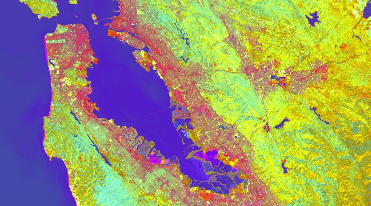
请注意,从数组图片中获取波段时,请先使用 project() 移除额外的维度,然后使用 arrayFlatten() 将其转换回常规图片。输出应如下所示: