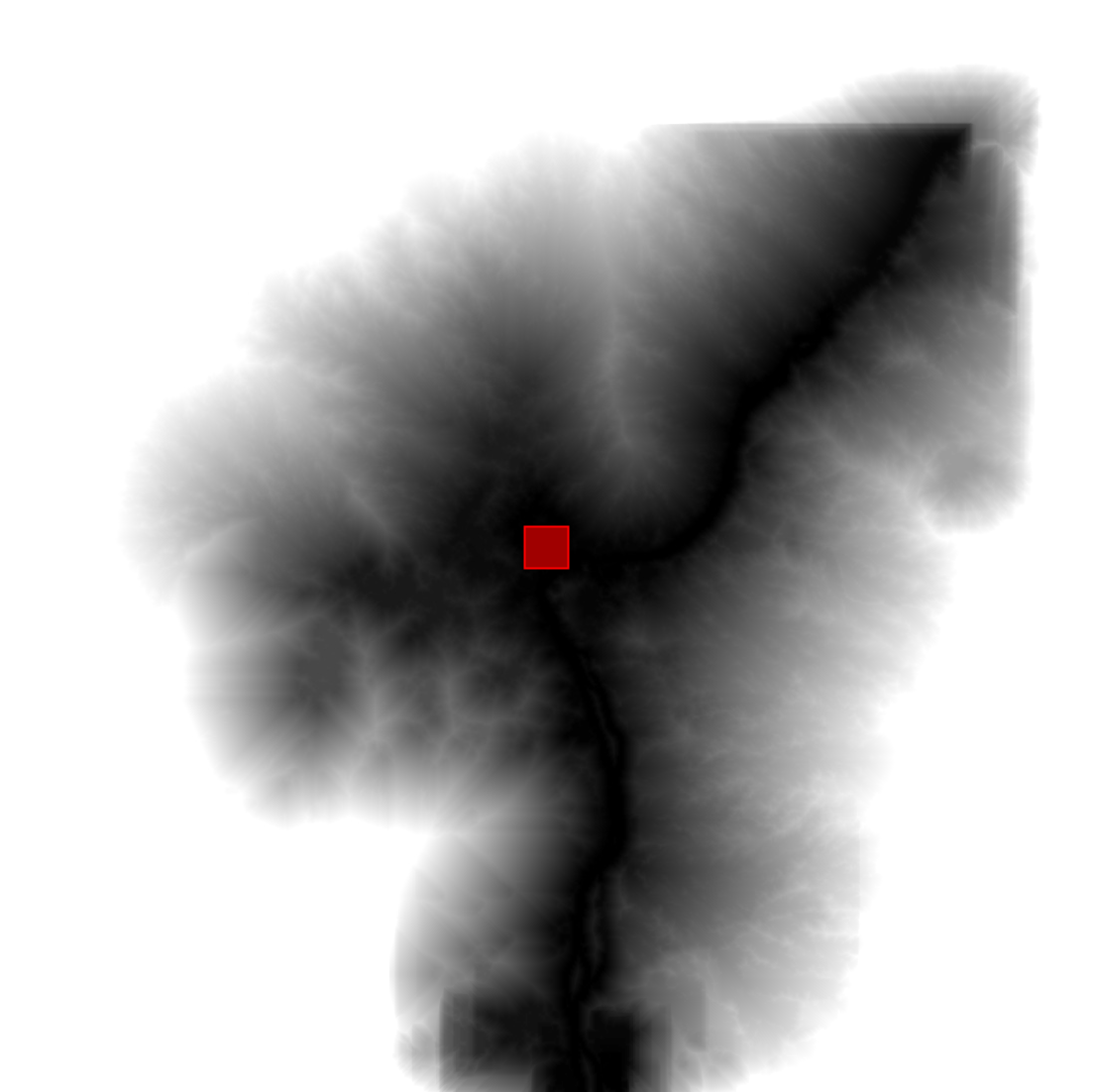
[null,null,["最后更新时间 (UTC):2025-07-25。"],[[["\u003cp\u003e\u003ccode\u003eimage.cumulativeCost()\u003c/code\u003e calculates the lowest-cost path from each pixel to the nearest source, useful for applications like habitat analysis, watershed delineation, and image segmentation.\u003c/p\u003e\n"],["\u003cp\u003eThe function requires a source image indicating starting points and a maximum distance for path calculation, considering the pixel resolution for accurate cost assessment.\u003c/p\u003e\n"],["\u003cp\u003eThe output image shows accumulated cost to the nearest source, with discontinuities appearing where the least-cost path exceeds the maximum distance.\u003c/p\u003e\n"],["\u003cp\u003eAn example demonstrates using land cover data to compute cumulative cost, visualizing the results on a map with source geometry and cost representation.\u003c/p\u003e\n"]]],[],null,["# Cumulative Cost Mapping\n\nUse `image.cumulativeCost()` to compute a cost map where every pixel\ncontains the total cost of the lowest cost path to the nearest source location. This\nprocess is useful in a variety of contexts such as habitat analysis\n[(Adriaensen\net al. 2003)](http://www.sciencedirect.com/science/article/pii/S0169204602002426), watershed delineation\n[(Melles et al.\n2011)](http://www.sciencedirect.com/science/article/pii/S1878029611001691) and image segmentation\n[(Falcao\net al. 2004).](http://ieeexplore.ieee.org/stamp/stamp.jsp?arnumber=1261076) Call the cumulative cost function on an image in which each pixel\nrepresents the cost per meter to traverse it. Paths are computed through any of a pixel's\neight neighbors. Required inputs include a `source` image, in which each\nnon-zero pixel represents a potential source (or start of a path), and a\n`maxDistance` (in meters) over which to compute paths. The algorithm finds\nthe cumulative cost of all paths less than *maxPixels* =\n`maxDistance`/*scale* in length, where *scale* is the pixel\nresolution, or [scale of analysis in Earth Engine](/earth-engine/guides/scale).\n\nThe following example demonstrates computing least-cost paths across a land cover\nimage:\n\n### Code Editor (JavaScript)\n\n```javascript\n// A rectangle representing Bangui, Central African Republic.\nvar geometry = ee.Geometry.Rectangle([18.5229, 4.3491, 18.5833, 4.4066]);\n\n// Create a source image where the geometry is 1, everything else is 0.\nvar sources = ee.Image().toByte().paint(geometry, 1);\n\n// Mask the sources image with itself.\nsources = sources.selfMask();\n\n// The cost data is generated from classes in ESA/GLOBCOVER.\nvar cover = ee.Image('ESA/GLOBCOVER_L4_200901_200912_V2_3').select(0);\n\n// Classes 60, 80, 110, 140 have cost 1.\n// Classes 40, 90, 120, 130, 170 have cost 2.\n// Classes 50, 70, 150, 160 have cost 3.\nvar beforeRemap = [60, 80, 110, 140,\n 40, 90, 120, 130, 170,\n 50, 70, 150, 160];\nvar afterRemap = [1, 1, 1, 1,\n 2, 2, 2, 2, 2,\n 3, 3, 3, 3];\nvar cost = cover.remap(beforeRemap, afterRemap, 0);\n\n// Compute the cumulative cost to traverse the land cover.\nvar cumulativeCost = cost.cumulativeCost({\n source: sources,\n maxDistance: 80 * 1000 // 80 kilometers\n});\n\n// Display the results\nMap.setCenter(18.71, 4.2, 9);\nMap.addLayer(cover, {}, 'Globcover');\nMap.addLayer(cumulativeCost, {min: 0, max: 5e4}, 'accumulated cost');\nMap.addLayer(geometry, {color: 'FF0000'}, 'source geometry');\n```\n\nThe result should look something like Figure 1, in which each output pixel represents the\naccumulated cost to the nearest source. Note that discontinuities can appear in places\nwhere the least cost path to the nearest source exceeds *maxPixels* in length.\nFigure 1. The cumulative cost to the source pixels, where cost is determined by the land cover categories. Low costs are black, higher costs are white."]]