Earth Engine 中的陣列是由數字清單和清單清單所組成。巢狀程度會決定維度的數量。如要從簡單的動機範例著手,請參考以下範例,瞭解如何使用 Landsat 8 纓帽 (TC) 係數建立 Array (Baig 等人,2014 年):
// Create an Array of Tasseled Cap coefficients.
var coefficients = ee.Array([
  [0.3029, 0.2786, 0.4733, 0.5599, 0.508, 0.1872],
  [-0.2941, -0.243, -0.5424, 0.7276, 0.0713, -0.1608],
  [0.1511, 0.1973, 0.3283, 0.3407, -0.7117, -0.4559],
  [-0.8239, 0.0849, 0.4396, -0.058, 0.2013, -0.2773],
  [-0.3294, 0.0557, 0.1056, 0.1855, -0.4349, 0.8085],
  [0.1079, -0.9023, 0.4119, 0.0575, -0.0259, 0.0252],
]);
import ee
import geemap.core as geemap
# Create an Array of Tasseled Cap coefficients.
coefficients = ee.Array([
    [0.3029, 0.2786, 0.4733, 0.5599, 0.508, 0.1872],
    [-0.2941, -0.243, -0.5424, 0.7276, 0.0713, -0.1608],
    [0.1511, 0.1973, 0.3283, 0.3407, -0.7117, -0.4559],
    [-0.8239, 0.0849, 0.4396, -0.058, 0.2013, -0.2773],
    [-0.3294, 0.0557, 0.1056, 0.1855, -0.4349, 0.8085],
    [0.1079, -0.9023, 0.4119, 0.0575, -0.0259, 0.0252],
])
確認這是使用 length() 的 6x6 2D 陣列,該函式會傳回每個軸的長度:
// Print the dimensions.
print(coefficients.length()); //    [6,6]
import ee
import geemap.core as geemap
# Print the dimensions.
display(coefficients.length())  #    [6,6]
下表說明矩陣項目沿著 0 軸和 1 軸的排列方式:
| 1 軸 -> | |||||||
|---|---|---|---|---|---|---|---|
| 0 | 1 | 2 | 3 | 4 | 5 | ||
| 0 | 0.3029 | 0.2786 | 0.4733 | 0.5599 | 0.508 | 0.1872 | |
| 1 | -0.2941 | -0.243 | -0.5424 | 0.7276 | 0.0713 | -0.1608 | |
| 0 軸 | 2 | 0.1511 | 0.1973 | 0.3283 | 0.3407 | -0.7117 | -0.4559 |
| 3 | -0.8239 | 0.0849 | 0.4396 | -0.058 | 0.2013 | -0.2773 | |
| 4 | -0.3294 | 0.0557 | 0.1056 | 0.1855 | -0.4349 | 0.8085 | |
| 5 | 0.1079 | -0.9023 | 0.4119 | 0.0575 | -0.0259 | 0.0252 | |
表格左側的索引代表沿著 0 軸的位移。0 軸上每個清單中的第 n 個元素,會位於 1 軸的第 n 個位置。舉例來說,陣列座標 [3,1] 的項目為 0.0849。假設「綠色」是感興趣的 TC 元件。您可以使用 slice() 取得綠度子矩陣:
// Get the 1x6 greenness slice, display it.
var greenness = coefficients.slice({axis: 0, start: 1, end: 2, step: 1});
print(greenness);
import ee
import geemap.core as geemap
# Get the 1x6 greenness slice, display it.
greenness = coefficients.slice(axis=0, start=1, end=2, step=1)
display(greenness)
2D 綠度矩陣應如下所示:
[[-0.2941,-0.243,-0.5424,0.7276,0.0713,-0.1608]]
請注意,slice() 的 start 和 end 參數對應至表格中顯示的 0 軸索引 (start 是包含,end 是排除)。
陣列圖片
如要取得綠度圖像,請將 Landsat 8 圖像的頻帶與綠度矩陣相乘。為此,請先將多波段 Landsat 圖像轉換為「陣列圖像」,其中每個像素都是一組波段值的 Array。例如:
// Load a Landsat 8 image, select the bands of interest.
var image = ee.Image('LANDSAT/LC08/C02/T1_TOA/LC08_044034_20140318')
  .select(['B2', 'B3', 'B4', 'B5', 'B6', 'B7']);

// Make an Array Image, with a 1-D Array per pixel.
var arrayImage1D = image.toArray();

// Make an Array Image with a 2-D Array per pixel, 6x1.
var arrayImage2D = arrayImage1D.toArray(1);
import ee
import geemap.core as geemap
# Load a Landsat 8 image, select the bands of interest.
image = ee.Image('LANDSAT/LC08/C02/T1_TOA/LC08_044034_20140318').select(
    ['B2', 'B3', 'B4', 'B5', 'B6', 'B7']
)

# Make an Array Image, with a 1-D Array per pixel.
array_image_1d = image.toArray()

# Make an Array Image with a 2-D Array per pixel, 6x1.
array_image_2d = array_image_1d.toArray(1)
請注意,在這個範例中,toArray() 會將 image 轉換為陣列圖片,其中每個像素都是 1 維向量,其項目對應於 image 頻帶中對應位置的 6 個值。以這種方式建立的 1 維向量陣列圖像,沒有 2D 形狀的概念。如要執行 2D 專屬作業 (例如矩陣相乘),請使用 toArray(1) 將其轉換為每個像素的 2D 陣列圖片。在 2D 陣列圖片的每個像素中,都有一個 6x1 矩陣的頻帶值。請參考以下玩具範例:
var array1D = ee.Array([1, 2, 3]);              // [1,2,3]
var array2D = ee.Array.cat([array1D], 1);     // [[1],[2],[3]]
import ee
import geemap.core as geemap
array_1d = ee.Array([1, 2, 3])  # [1,2,3]
array_2d = ee.Array.cat([array_1d], 1)  # [[1],[2],[3]]
請注意,array1D 向量會沿著 0 軸變化。array2D 矩陣也是如此,但它有額外的維度。對陣列圖片呼叫 toArray(1) 就像對每個像素呼叫 cat(bandVector, 1)。使用 2D 陣列圖片,左乘圖片,其中每個像素都包含綠度係數的 2D 矩陣:
// Do a matrix multiplication: 1x6 times 6x1.
// Cast the greenness Array to an Image prior to multiplication.
var greennessArrayImage = ee.Image(greenness).matrixMultiply(arrayImage2D);
import ee
import geemap.core as geemap
# Do a matrix multiplication: 1x6 times 6x1.
# Cast the greenness Array to an Image prior to multiplication.
greenness_array_image = ee.Image(greenness).matrixMultiply(array_image_2d)
結果是新的陣列圖片,其中每個像素都是 1x1 矩陣,是矩陣相乘 1x6 綠度矩陣 (左側) 和 6x1 頻帶矩陣 (右側) 的結果。如要顯示圖片,請使用 arrayGet() 轉換為一般單頻帶圖片:
// Get the result from the 1x1 array in each pixel of the 2-D array image.
var greennessImage = greennessArrayImage.arrayGet([0, 0]);

// Display the input imagery with the greenness result.
Map.setCenter(-122.3, 37.562, 10);
Map.addLayer(image, {bands: ['B5', 'B4', 'B3'], min: 0, max: 0.5}, 'image');
Map.addLayer(greennessImage, {min: -0.1, max: 0.13}, 'greenness');
import ee
import geemap.core as geemap
# Get the result from the 1x1 array in each pixel of the 2-D array image.
greenness_image = greenness_array_image.arrayGet([0, 0])

# Display the input imagery with the greenness result.
m = geemap.Map()
m.set_center(-122.3, 37.562, 10)
m.add_layer(image, {'bands': ['B5', 'B4', 'B3'], 'min': 0, 'max': 0.5}, 'image')
m.add_layer(greenness_image, {'min': -0.1, 'max': 0.13}, 'greenness')
m
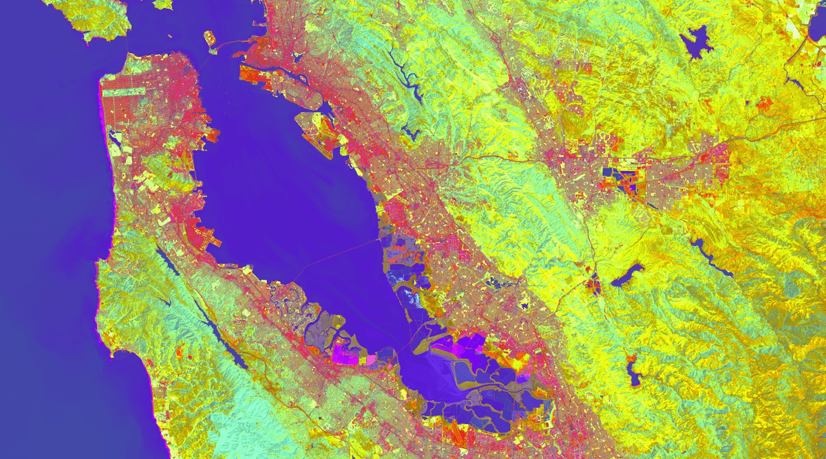
以下是完整範例,其中使用整個係數陣列一次計算多個纓穗圓頂元件並顯示結果:
// Define an Array of Tasseled Cap coefficients.
var coefficients = ee.Array([
  [0.3029, 0.2786, 0.4733, 0.5599, 0.508, 0.1872],
  [-0.2941, -0.243, -0.5424, 0.7276, 0.0713, -0.1608],
  [0.1511, 0.1973, 0.3283, 0.3407, -0.7117, -0.4559],
  [-0.8239, 0.0849, 0.4396, -0.058, 0.2013, -0.2773],
  [-0.3294, 0.0557, 0.1056, 0.1855, -0.4349, 0.8085],
  [0.1079, -0.9023, 0.4119, 0.0575, -0.0259, 0.0252],
]);

// Load a Landsat 8 image, select the bands of interest.
var image = ee.Image('LANDSAT/LC08/C02/T1_TOA/LC08_044034_20140318')
  .select(['B2', 'B3', 'B4', 'B5', 'B6', 'B7']);

// Make an Array Image, with a 1-D Array per pixel.
var arrayImage1D = image.toArray();

// Make an Array Image with a 2-D Array per pixel, 6x1.
var arrayImage2D = arrayImage1D.toArray(1);

// Do a matrix multiplication: 6x6 times 6x1.
var componentsImage = ee.Image(coefficients)
  .matrixMultiply(arrayImage2D)
  // Get rid of the extra dimensions.
  .arrayProject([0])
  .arrayFlatten(
    [['brightness', 'greenness', 'wetness', 'fourth', 'fifth', 'sixth']]);

// Display the first three bands of the result and the input imagery.
var vizParams = {
  bands: ['brightness', 'greenness', 'wetness'],
  min: -0.1, max: [0.5, 0.1, 0.1]
};
Map.setCenter(-122.3, 37.562, 10);
Map.addLayer(image, {bands: ['B5', 'B4', 'B3'], min: 0, max: 0.5}, 'image');
Map.addLayer(componentsImage, vizParams, 'components');
import ee
import geemap.core as geemap
# Define an Array of Tasseled Cap coefficients.
coefficients = ee.Array([
    [0.3029, 0.2786, 0.4733, 0.5599, 0.508, 0.1872],
    [-0.2941, -0.243, -0.5424, 0.7276, 0.0713, -0.1608],
    [0.1511, 0.1973, 0.3283, 0.3407, -0.7117, -0.4559],
    [-0.8239, 0.0849, 0.4396, -0.058, 0.2013, -0.2773],
    [-0.3294, 0.0557, 0.1056, 0.1855, -0.4349, 0.8085],
    [0.1079, -0.9023, 0.4119, 0.0575, -0.0259, 0.0252],
])

# Load a Landsat 8 image, select the bands of interest.
image = ee.Image('LANDSAT/LC08/C02/T1_TOA/LC08_044034_20140318').select(
    ['B2', 'B3', 'B4', 'B5', 'B6', 'B7']
)

# Make an Array Image, with a 1-D Array per pixel.
array_image_1d = image.toArray()

# Make an Array Image with a 2-D Array per pixel, 6x1.
array_image_2d = array_image_1d.toArray(1)

# Do a matrix multiplication: 6x6 times 6x1.
components_image = (
    ee.Image(coefficients)
    .matrixMultiply(array_image_2d)
    # Get rid of the extra dimensions.
    .arrayProject([0])
    .arrayFlatten(
        [['brightness', 'greenness', 'wetness', 'fourth', 'fifth', 'sixth']]
    )
)

# Display the first three bands of the result and the input imagery.
viz_params = {
    'bands': ['brightness', 'greenness', 'wetness'],
    'min': -0.1,
    'max': [0.5, 0.1, 0.1],
}
m = geemap.Map()
m.set_center(-122.3, 37.562, 10)
m.add_layer(image, {'bands': ['B5', 'B4', 'B3'], 'min': 0, 'max': 0.5}, 'image')
m.add_layer(components_image, viz_params, 'components')
m
請注意,從陣列圖片取得頻帶時,請先使用 project() 移除額外的維度,然後再使用 arrayFlatten() 將其轉換回一般圖片。輸出內容應如下所示: