이미지 컬렉션은 Earth Engine 이미지 세트를 의미합니다. 예를 들어 모든 Landsat 8 이미지의 컬렉션은 ee.ImageCollection입니다. 지금까지 사용한 SRTM 이미지와 마찬가지로 이미지 컬렉션에도 ID가 있습니다. 단일 이미지와 마찬가지로 코드 편집기에서 Earth Engine 데이터 카탈로그를 검색하고 데이터 세트의 세부정보 페이지를 확인하여 이미지 컬렉션의 ID를 찾을 수 있습니다. 예를 들어 'landsat 8 toa'를 검색하고 첫 번째 결과를 클릭합니다. 이 결과는
USGS Landsat 8 Collection 1 Tier 1 TOA Reflectance 데이터 세트에 해당합니다.
가져오기 버튼을 사용하여 데이터 세트를 가져오고 l8로 이름을 바꾸거나 ID를 이미지 컬렉션 생성자에 복사합니다.
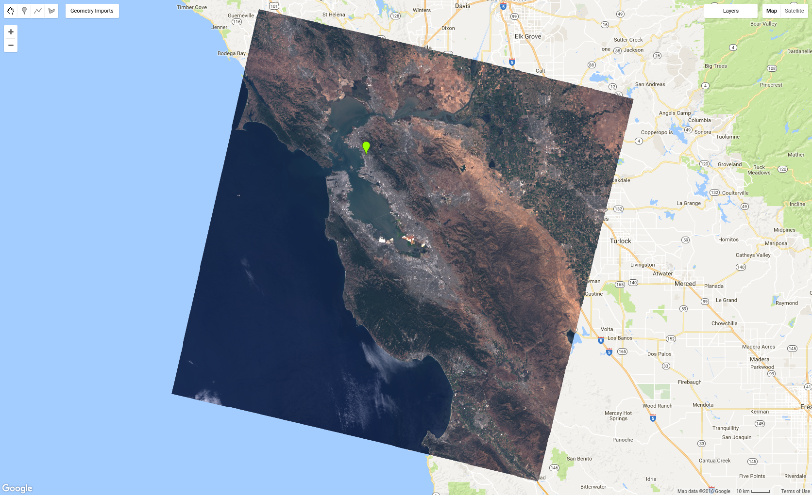
이 컬렉션은 전 세계에서 수집된 모든 Landsat 8 장면을 나타냅니다. 알고리즘을 테스트할 단일 이미지 또는 이미지 하위 집합을 추출하는 것이 유용한 경우가 많습니다. 시간 또는 공간별로 수집을 제한하는 방법은 필터링하는 것입니다. 예를 들어 특정 위치를 포함하는 이미지로 컬렉션을 필터링하려면 먼저 도형 그리기 도구를 사용하여 점 (또는 선이나 다각형)으로 관심 영역을 정의합니다. 관심 영역으로 이동하고 지오메트리 가져오기에 마우스를 가져간 후 (이미 하나 이상의 지오메트리가 정의된 경우) +새 레이어를 클릭합니다 (가져오기가 없는 경우 다음 단계로 이동). 포인트 그리기 도구()를 가져와 관심 영역에 포인트를 만듭니다. 가져오기 이름을 point로 지정합니다. 이제 l8 컬렉션을 필터링하여 점과 교차하는 이미지만 가져온 다음 두 번째 필터를 추가하여 컬렉션을 2015년에 획득한 이미지로만 제한합니다.
여기서 filterBounds() 및 filterDate()은 이미지 컬렉션의 더 일반적인 filter() 메서드의 바로가기 메서드이며, ee.Filter()을 인수로 사용합니다. 코드 편집기의 문서 탭을 살펴보고 이러한 메서드에 대해 자세히 알아보세요. filterBounds()의 인수는 디지털화한 포인트이고 filterDate()의 인수는 문자열로 표현된 두 날짜입니다.
필터링된 컬렉션을 print()할 수 있습니다. 한 번에 5,000개 이상의 항목을 인쇄할 수 없으므로 l8 전체 컬렉션을 인쇄할 수는 없습니다. print() 메서드를 실행한 후 콘솔에서 인쇄된 컬렉션을 검사할 수 있습니다. 지퍼()를 사용하여 ImageCollection를 펼친 다음 features 목록을 펼치면 이미지 목록이 표시되며 각 이미지를 펼쳐 검사할 수도 있습니다. 개별 이미지의 ID를 찾는 한 가지 방법입니다. 분석을 위해 개별 이미지를 가져오는 또 다른 프로그래매틱 방식은 일부 메타데이터 속성과 관련하여 가장 최근, 가장 오래된 또는 최적의 이미지를 가져오기 위해 컬렉션을 정렬하는 것입니다. 예를 들어 인쇄된 이미지 컬렉션의 이미지 객체를 검사하면 CLOUD_COVER라는 메타데이터 속성이 표시될 수 있습니다. 이 속성을 사용하여 관심 지역에서 2015년에 구름이 가장 적은 이미지를 가져올 수 있습니다.
코드 편집기 (JavaScript)
// This will sort from least to most cloudy.varsorted=temporalFiltered.sort('CLOUD_COVER');// Get the first (least cloudy) image.varscene=sorted.first();
이제 이미지를 표시할 수 있습니다.
여담: RGB 이미지 표시
멀티밴드 이미지가 지도에 추가되면 Earth Engine은 이미지의 처음 세 개 밴드를 선택하고 데이터 유형에 따라 앞서 설명한 대로 늘려 기본적으로 빨간색, 녹색, 파란색으로 표시합니다. 일반적으로는 이렇게 하면 안 됩니다. 예를 들어 이전 예의 Landsat 이미지(scene)를 지도에 추가하면 결과가 만족스럽지 않습니다.
먼저 지도가 확대/축소 비율 9에서 이미지의 중앙에 배치됩니다. 그러면 이미지가 visParams 매개변수에 대해 빈 객체 ({})와 함께 표시됩니다(자세한 내용은 Map.addLayer() 문서를 참고하세요). 따라서 이미지는 기본 시각화로 표시됩니다. 처음 세 개의 밴드는 각각 R, G, B에 매핑되고 밴드가 float 데이터 유형이므로 [0, 1] 로 늘어납니다. 즉, 연안 에어로졸 밴드 ('B1')는 빨간색으로 렌더링되고, 파란색 밴드 ('B2')는 녹색으로 렌더링되며, 녹색 밴드 ('B3')는 파란색으로 렌더링됩니다. 이미지를 트루 컬러 컴포지트로 렌더링하려면 Earth Engine에 Landsat 8 밴드 'B4', 'B3', 'B2'를 각각 R, G, B에 사용하도록 지시해야 합니다. visParams 객체의 bands 속성과 함께 사용할 밴드를 지정합니다. 이 참조에서 Landsat 대역에 대해 자세히 알아보세요.
일반적인 지구 표면 타겟의 반사율을 표시하는 데 적합한 min 및 max 값도 제공해야 합니다. 목록을 사용하여 각 대역의 다른 값을 지정할 수 있지만 여기서는 0.3를 max로 지정하고 min 매개변수의 기본값인 0을 사용하면 됩니다. 시각화 매개변수를 하나의 객체로 결합하고 표시합니다.
이제 축소하면 Landsat 이미지가 수집된 연속 모자이크 (즉, 육지 위)를 볼 수 있습니다. 인스펙터 탭을 사용하여 이미지를 클릭하면 픽셀 섹션에 픽셀 값 목록 (또는 차트)이 표시되고 인스펙터의 객체 섹션에 이미지 객체 목록이 표시됩니다.
충분히 확대하면 모자이크에 구름이 표시되는 것을 알 수 있습니다. 지도에 ImageCollection를 추가하면 최근 값 컴포지트가 표시됩니다. 즉, 가장 최근 픽셀만 표시됩니다 (컬렉션에서 mosaic()를 호출하는 것과 같음). 따라서 서로 다른 시간에 획득한 경로 사이에 불연속이 표시될 수 있습니다. 이로 인해 많은 지역이 흐리게 표시될 수 있습니다. 다음 페이지에서 이미지가 합성되는 방식을 변경하여 성가신 구름을 없애는 방법을 알아보세요.
[null,null,["최종 업데이트: 2025-07-27(UTC)"],[[["\u003cp\u003eAn \u003ccode\u003eee.ImageCollection\u003c/code\u003e in Earth Engine represents a set of images, such as all Landsat 8 images, and can be filtered by location and date.\u003c/p\u003e\n"],["\u003cp\u003eIndividual images within a collection can be accessed by sorting based on metadata properties like cloud cover, allowing selection of specific images.\u003c/p\u003e\n"],["\u003cp\u003eDisplaying images requires specifying visualization parameters, like bands for RGB composites and stretching values, for optimal visualization.\u003c/p\u003e\n"],["\u003cp\u003eImage collections can be added to the map, displayed as recent-value composites, showing the most recent pixels and potential cloud cover.\u003c/p\u003e\n"],["\u003cp\u003eEarth Engine's capabilities extend beyond single scenes, enabling large-scale analyses using entire image collections and advanced compositing techniques.\u003c/p\u003e\n"]]],[],null,["# Image Collections\n\nAn image collection refers to a set of Earth Engine images. For example, the collection\nof all Landsat 8 images is an `ee.ImageCollection`. Like the SRTM image\nyou have been working with, image collections also have an ID. As with single images,\nyou can discover the ID of an image collection by searching the\n[Earth Engine data catalog](/earth-engine/datasets) from\nthe Code Editor and looking at the details page of the dataset. For example, search for\n'landsat 8 toa' and click on the first result, which should correspond to the\n[USGS Landsat 8 Collection 1 Tier 1 TOA Reflectance](https://developers.google.com/earth-engine/datasets/catalog/LANDSAT_LC08_C01_T1_TOA) dataset.\nEither import that dataset using the **Import** button and rename it to `l8`, or copy the ID into the\nimage collection constructor:\n\n### Code Editor (JavaScript)\n\n```javascript\nvar l8 = ee.ImageCollection('LANDSAT/LC08/C02/T1_TOA');\n```\n\nFiltering image collections\n---------------------------\n\nIt's worth noting that this collection represents *every* Landsat 8 scene collected,\nall over the Earth. Often it is useful to extract a single image, or subset of images,\non which to test algorithms. The way to limit the collection by time or space is by\nfiltering it. For example, to filter the collection to images that cover a particular\nlocation, first define your area of interest\nwith a point (or line or polygon) using the geometry drawing tools. Pan to your area of\ninterest, hover on the **Geometry Imports** (if you already have one or more\ngeometries defined) and click **+new layer** (if you don't have any imports,\ngo to the next step). Get the point drawing tool\n() and make a point in your area of\ninterest. Name the import `point`. Now, filter the `l8` collection\nto get *only* the images that intersect the point, then add a second filter to\nlimit the collection to only the images that were acquired in 2015:\n\n### Code Editor (JavaScript)\n\n```javascript\nvar spatialFiltered = l8.filterBounds(point);\nprint('spatialFiltered', spatialFiltered);\n\nvar temporalFiltered = spatialFiltered.filterDate('2015-01-01', '2015-12-31');\nprint('temporalFiltered', temporalFiltered);\n```\n\nHere, `filterBounds()` and `filterDate()` are shortcut methods for\nthe more general `filter()` method on image collections, which takes an\n`ee.Filter()` as its argument. Explore the **Docs** tab of the Code\nEditor to learn more about these methods. The argument to `filterBounds()`\nis the point you digitized and the arguments to `filterDate()` are two dates,\nexpressed as strings.\n\nNote that you can `print()` the filtered collections. You can't print more than\n5000 things at once, so you couldn't, for example, print the entire `l8`\ncollection. After executing the `print()` method, you can inspect the\nprinted collections in the console. Note that when you expand the\n`ImageCollection` using the zippy\n(), then expand the\nlist of `features`, you will see a list of images, each of which also can be\nexpanded and inspected. This is one way to discover the ID of an individual image. Another,\nmore programmatic way to get individual images for analysis is to sort the collection\nin order to get the most recent, oldest, or optimal image relative to some metadata\nproperty. For example, by inspecting the image objects in the printed image collections,\nyou may have observed a metadata property called `CLOUD_COVER`. You can use\nthat property to get the least cloudy image in 2015 in your area of interest:\n\n\n### Code Editor (JavaScript)\n\n```javascript\n// This will sort from least to most cloudy.\nvar sorted = temporalFiltered.sort('CLOUD_COVER');\n\n// Get the first (least cloudy) image.\nvar scene = sorted.first();\n```\n\nYou're now ready to display the image!\n\nDigression: Displaying RGB images\n---------------------------------\n\nWhen a multi-band image is added to a map, Earth Engine chooses the first three bands of\nthe image and displays them as red, green, and blue by default, stretching them according\nto the data type, [as described\npreviously](/earth-engine/tutorials/tutorial_api_02#digression-images-in-earth-engine). Usually, this won't do. For example, if you add the Landsat image\n(`scene` in the previous example) to the map, the result is unsatisfactory:\n\n### Code Editor (JavaScript)\n\n```javascript\nMap.centerObject(scene, 9);\nMap.addLayer(scene, {}, 'default RGB');\n```\n\nNote that first, the map is centered on the image at zoom scale 9. Then the image is\ndisplayed with an empty object (`{}`) for the `visParams` parameter\n(see the `Map.addLayer()` docs for details). As a result, the image is\ndisplayed with the default visualization: first three bands map to R, G, B, respectively,\nand stretched to \\[0, 1\\] since the bands are `float` data type. This means that\nthe coastal aerosol band ('B1') is rendered in red, the blue band ('B2') is rendered\nin green, and the green band ('B3') is rendered in blue. To render the image as a\ntrue-color composite, you need to tell Earth Engine to use the Landsat 8 bands 'B4', 'B3',\nand 'B2' for R, G, and B, respectively. Specify which bands to use with the\n`bands` property of the `visParams` object. Learn more about\nLandsat bands at\n[this\nreference](https://www.usgs.gov/faqs/what-are-band-designations-landsat-satellites).\n\nYou also need to provide `min` and `max` values suitable for\ndisplaying reflectance from typical Earth surface targets. Although lists can be used to\nspecify different values for each band, here it's sufficient to\nspecify `0.3` as `max` and use the default value of zero for the\n`min` parameter. Combining the visualization parameters into one object and\ndisplaying:\n\n### Code Editor (JavaScript)\n\n```javascript\nvar visParams = {bands: ['B4', 'B3', 'B2'], max: 0.3};\nMap.addLayer(scene, visParams, 'true-color composite');\n```\n\nThe result should look something like Figure 5. Note that this code assigns the object\nof visualization parameters to a variable for possible future use. As you'll soon\ndiscover, that object will be useful when you visualize image collections!\nFigure 5. Landsat 8 TOA reflectance image as a true-color composite, stretched to \\[0, 0.3\\].\n\nTry playing with visualizing different bands. Another favorite combination is 'B5', 'B4',\nand 'B3' which is called a false-color composite. Some other interesting false-color\ncomposites are described\n[here](https://www.usgs.gov/media/images/common-landsat-band-rgb-composites).\n\nSince Earth Engine is designed to do large-scale analyses, you are not limited to working\nwith just one scene. Now it's time to display a whole collection as an RGB composite!\n\nDisplaying image collections\n----------------------------\n\nAdding an image collection to a map is similar to adding an image to a map. For\nexample, using 2016 images in the `l8` collection and the `visParams`\nobject defined previously,\n\n### Code Editor (JavaScript)\n\n```javascript\nvar l8 = ee.ImageCollection('LANDSAT/LC08/C02/T1_TOA');\nvar landsat2016 = l8.filterDate('2016-01-01', '2016-12-31');\nMap.addLayer(landsat2016, visParams, 'l8 collection');\n```\n\nNote that now you can zoom out and see a continuous mosaic where Landsat imagery\nis collected (i.e. over land). Also note that when you use the **Inspector**\ntab and click on the image, you'll see a list of pixel values (or a chart) in the\n**Pixels** section and a list of image objects in the **Objects**\nsection of the inspector.\n\nIf you zoomed out enough, you probably noticed some clouds in the mosaic. When\nyou add an `ImageCollection` to the map, it is displayed as a recent-value\ncomposite, meaning that only the most recent pixels are displayed (like calling\n`mosaic()` on the collection). That is why you can see discontinuities between\n[paths](http://landsat.gsfc.nasa.gov/?p=3231) which were acquired at\ndifferent times. It's also why many areas may appear cloudy. In the next page, learn how\nto change the way the images are composited to get rid of those pesky clouds! \n[arrow_backPrevious page](/earth-engine/tutorials/tutorial_api_03) [Next pagearrow_forward](/earth-engine/tutorials/tutorial_api_05)"]]